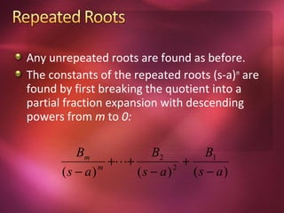
Downloaded 342 times

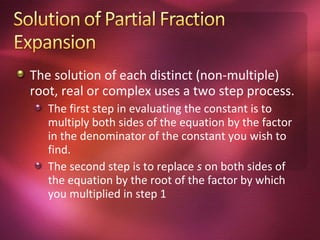
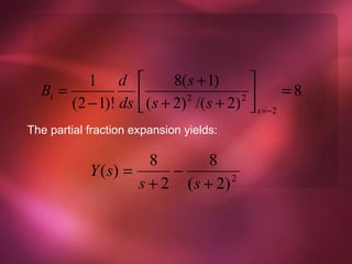

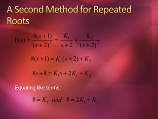
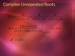
![8( s + 1) 2 K1 8
( s + 2)
2
= ( s + 2) − ( s + 2) 2
( s + 2) 2
s+2 ( s + 2) 2
d [ 8( s + 1)] d [ ( s + 2 ) K1 − 8]
=
ds ds
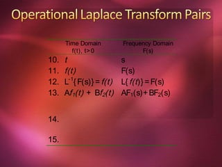
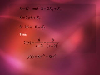
8 = K1
8( s + 1) 8 8
Y (s) = = −
( s + 2) 2
s + 2 ( s + 2) 2
y (t ) = 8e −2t − 8te −2t](https://image.slidesharecdn.com/laplace-121103114837-phpapp01/85/Laplace-transformation-26-320.jpg)

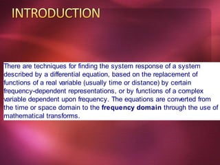
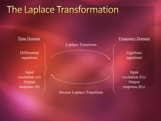
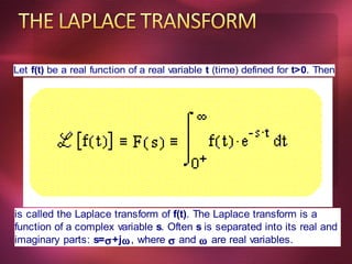
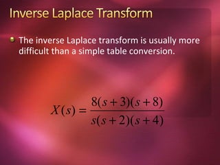
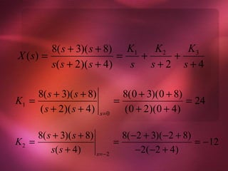
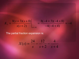
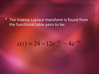
1. The Laplace transform converts differential equations describing systems from the time domain to the frequency domain by replacing functions of time with functions of a complex variable dependent on frequency. 2. The inverse Laplace transform converts the solution back from the frequency domain to the time domain to obtain the solution in terms of the time variable. 3. Partial fraction expansion is often used to break solutions into simpler terms that can be inverted using Laplace transform tables to find the solution in the time domain.