This document provides an overview of functional analysis concepts including:
1. It defines metric spaces and provides examples of metric spaces such as Rn with the Euclidean metric and function spaces with supremum metrics.
2. It introduces concepts for metric spaces like open and closed sets, continuous mappings, accumulation points, and separable spaces.
3. It defines convergence of sequences in metric spaces and Cauchy sequences, and introduces the concept of completeness of metric spaces.
4. The document continues by discussing normed spaces, linear operators, bounded linear operators, linear functionals, and dual spaces.
5. It also covers Hilbert spaces, fundamental theorems in functional analysis like the open mapping theorem and closed
![Functional Analysis
July 12, 2007
Contents
1 Metric Spaces 3
1.1 Open Sets, Closed Sets . . . . . . . . . . . . . . . . . . . . . . . . . . . . . . 5
1.2 Convergence, Cauchy Sequence, Completeness . . . . . . . . . . . . . . . . . 7
1.3 Completeness Proofs . . . . . . . . . . . . . . . . . . . . . . . . . . . . . . . 9
1.4 Completion of Metric Spaces . . . . . . . . . . . . . . . . . . . . . . . . . . 10
2 Normed Spaces 13
2.1 Finite dimensional Normed Spaces or Subspaces . . . . . . . . . . . . . . . 15
2.2 Compactness and Finite Dimension . . . . . . . . . . . . . . . . . . . . . . . 18
2.3 Linear Operators . . . . . . . . . . . . . . . . . . . . . . . . . . . . . . . . . 22
2.4 Bounded and Continuous Linear Operators . . . . . . . . . . . . . . . . . . 24
2.5 Linear Functionals . . . . . . . . . . . . . . . . . . . . . . . . . . . . . . . . 29
2.6 Finite Dimensional Case . . . . . . . . . . . . . . . . . . . . . . . . . . . . . 32
2.6.1 Linear Functionals . . . . . . . . . . . . . . . . . . . . . . . . . . . . 33
2.7 Dual Space . . . . . . . . . . . . . . . . . . . . . . . . . . . . . . . . . . . . 35
3 Hilbert Spaces 39
3.1 Representation of Functionals on Hilbert Spaces . . . . . . . . . . . . . . . 49
3.2 Hilbert Adjoint . . . . . . . . . . . . . . . . . . . . . . . . . . . . . . . . . . 53
4 Fundamental Theorems 59
4.1 Bounded, Linear Functionals on C[a, b] . . . . . . . . . . . . . . . . . . . . . 68
4.2 Adjoint Operator . . . . . . . . . . . . . . . . . . . . . . . . . . . . . . . . . 71
4.3 Reflexive Spaces . . . . . . . . . . . . . . . . . . . . . . . . . . . . . . . . . 75
4.4 Baire Category Theorem . . . . . . . . . . . . . . . . . . . . . . . . . . . . . 78
4.5 Strong and Weak Convergence . . . . . . . . . . . . . . . . . . . . . . . . . 81
4.6 The Open Mapping Theorem . . . . . . . . . . . . . . . . . . . . . . . . . . 88
4.7 Closed Graph Theorem . . . . . . . . . . . . . . . . . . . . . . . . . . . . . 89
1](https://image.slidesharecdn.com/notes-121009204506-phpapp01/85/Notes-1-320.jpg)
![Functional Analysis
July 12, 2007
Contents
1 Metric Spaces 3
1.1 Open Sets, Closed Sets . . . . . . . . . . . . . . . . . . . . . . . . . . . . . . 5
1.2 Convergence, Cauchy Sequence, Completeness . . . . . . . . . . . . . . . . . 7
1.3 Completeness Proofs . . . . . . . . . . . . . . . . . . . . . . . . . . . . . . . 9
1.4 Completion of Metric Spaces . . . . . . . . . . . . . . . . . . . . . . . . . . 10
2 Normed Spaces 13
2.1 Finite dimensional Normed Spaces or Subspaces . . . . . . . . . . . . . . . 15
2.2 Compactness and Finite Dimension . . . . . . . . . . . . . . . . . . . . . . . 18
2.3 Linear Operators . . . . . . . . . . . . . . . . . . . . . . . . . . . . . . . . . 22
2.4 Bounded and Continuous Linear Operators . . . . . . . . . . . . . . . . . . 24
2.5 Linear Functionals . . . . . . . . . . . . . . . . . . . . . . . . . . . . . . . . 29
2.6 Finite Dimensional Case . . . . . . . . . . . . . . . . . . . . . . . . . . . . . 32
2.6.1 Linear Functionals . . . . . . . . . . . . . . . . . . . . . . . . . . . . 33
2.7 Dual Space . . . . . . . . . . . . . . . . . . . . . . . . . . . . . . . . . . . . 35
3 Hilbert Spaces 39
3.1 Representation of Functionals on Hilbert Spaces . . . . . . . . . . . . . . . 49
3.2 Hilbert Adjoint . . . . . . . . . . . . . . . . . . . . . . . . . . . . . . . . . . 53
4 Fundamental Theorems 59
4.1 Bounded, Linear Functionals on C[a, b] . . . . . . . . . . . . . . . . . . . . . 68
4.2 Adjoint Operator . . . . . . . . . . . . . . . . . . . . . . . . . . . . . . . . . 71
4.3 Reflexive Spaces . . . . . . . . . . . . . . . . . . . . . . . . . . . . . . . . . 75
4.4 Baire Category Theorem . . . . . . . . . . . . . . . . . . . . . . . . . . . . . 78
4.5 Strong and Weak Convergence . . . . . . . . . . . . . . . . . . . . . . . . . 81
4.6 The Open Mapping Theorem . . . . . . . . . . . . . . . . . . . . . . . . . . 88
4.7 Closed Graph Theorem . . . . . . . . . . . . . . . . . . . . . . . . . . . . . 89
1](https://image.slidesharecdn.com/notes-121009204506-phpapp01/75/Notes-1-2048.jpg)

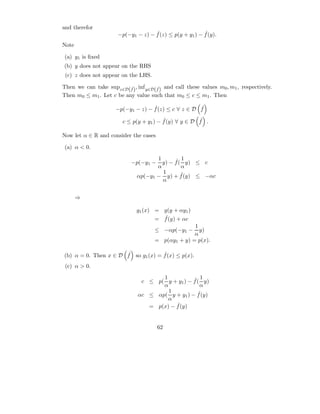
![1 Metric Spaces
Definition (Metric Space). The pair (X, d), where X is a set and the function
d:X ×X →R
is called a metric space if
1. d(x, y) ≥ 0
2. d(x, y) = 0 iff x = y
3. d(x, y) = d(y, x)
4. d(x, y) ≤ d(x, z) + d(z, y)
Example 1.1 (Metric Spaces).
1. d(x, y) = |x − y| in R.
n 1
2. d(x, y) = [ i=1 (xi − yi )2 ] 2 in Rn .
3. d(x, y) = x − y in a normed space.
4. Let (X, ρ), (Y, σ) be metric spaces and define the Cartesian product X × Y =
{(x, y)|x ∈ X, y ∈ Y }. Then the product measure τ ((x1 , y1 ), (x2 , y2 )) = [ρ(x1 , x2 )2 +
1
σ(y1 , y2 )2 ] 2 .
¯ ¯
5. (Subspace) (Y, d) of (X, d) if Y ⊂ X and d = d|Y ×Y .
6. l∞ . Let X be the set of all bounded sequences of complex numbers, i.e., x =
(ξi ) and |ξi | ≤ cx , ∀ i. Then
d(x, y) = sup |ξi − ηi |
i∈N
defines a metric on X.
7. X = C[a, b] and
d(x, y) = max |x(t) − y(t)|.
t∈[a,b]
8. (Discrete metric)
1 x=y
d(x, y) = .
0 x=y
3](https://image.slidesharecdn.com/notes-121009204506-phpapp01/85/Notes-3-320.jpg)
![∞
9. lp . x = (ξi ) ∈ lp if i=1 |ξi |
p < ∞, (p ≥ 1, fixed),
1
∞ p
d(x, y) = |ξi − ηi |p .
i=1
Problem 1.
¯
1. Show that d is a metric on C[a, b], where
b
¯
d(x, y) = |x(t) − y(t)|dt.
a
2. Show that the discrete metric is a metric.
3. Sequence space s: set of all sequences of complex numbers with the metric
∞
1 |ξi − ηi |
d(x, y) = . (1)
2i 1 + |ξi − ηi |
i=1
Solution.
¯
1. d(x, y) = 0 iff |x(t) − y(t)| = 0 for all t ∈ [a, b] because of the continuity. We have
¯ ¯ ¯
d(x, y) ≥ 0 and d(x, y) = d(y, x) trivially. We can argue the triangle inequality as
follows::
b b b
¯
d(x, y) = |x(t) − y(t)|dt ≤ |x(t) − z(t)|dt + ¯ ¯
|z(t) − y(t)|dt = d(x, z) + d(z, y).
a a a
2. Left as an exercise.
3. We show only the triangle inequality. Let a, b ∈ R. Then we have the inequalities
|a + b| |a| + |b| |a| |b|
≤ ≤ + ,
1 + |a + b| 1 + |a| + |b| 1 + |a| 1 + |b|
where in the first step we have used the monotonicity of the function
x 1
f (x) = =1− , for x > 0.
1+x 1+x
Substituting a = ξi − ζi and b = ζi − ηi , where x = (ξi ), y = (ηi ), and z = (ζi ) we get
|ξi − ηi | |ξi − ζi | |ζi − ηi |
≤ + .
1 + |ξi − ηi | 1 + |ξi − ζi | 1 + |ζi − ηi |
1
If we multiply both sides by 2i
and sum over from i = 1 to ∞ we get the stated
result.
4](https://image.slidesharecdn.com/notes-121009204506-phpapp01/85/Notes-4-320.jpg)
![1.3 Completeness Proofs
Theorem 1.12. Rn , Cn are complete.
Theorem 1.13. ℓ∞ is complete.
Proof. Let (xm ) be a Cauchy sequence in ℓ∞ .
(m) (n)
⇒ d(xm , xn ) = sup |xi − xi | < ε, for m, n > N (ε).
i
(m) (m)
⇒ for fixed i, the sequence (ξi ) is Cauchy in R, and therefore we have that ξi →
ξi , for i = 1, 2, 3, ... Let x = (ξi ). It follows easily that x ∈ ℓ∞ and xm → x.
Theorem 1.14. The space of convergent sequences x = (ξi ) of complex numbers with the
metric induced from ℓ∞ is complete.
Theorem 1.15. ℓp is complete if 1 ≤ p < ∞.
Theorem 1.16. C[a, b] is complete.
Proof. Let (xm ) be a Cauchy sequence in C[a, b]. Then
∀ ε > 0 ∃ N s.t. for m, n > N ⇒ d(xm , xn ) = max |xm (t) − xn (t)| < ε. (2)
t∈[a,b]
⇒ for any fixed t0 ∈ [a, b] we have that |xm (t0 ) − xn (t0 )| < ε. It follows that xm (t0 ) is
Cauchy and therefore xm (t0 ) → x(t0 ). Show that x(t) ∈ C[a, b] and xm → x. From (2)
with n → ∞ we get
max |xm (t) − x(t)| ≤ ε.
t∈[a,b]
Therefore xm (t) converges uniformly to x(t) on [a, b]. Since the xm ’s are continuous on
[a, b] and the convergence is uniform x(t) is continuous, and thus belongs to C[a, b].
Remark 1.17. Note that in C[a, b] convergence is uniform convergence; we also use the
terminology uniform metric for the metric generated by the “sup”-norm.
Example 1.18 (Incomplete Metric Spaces).
1. Q
2. The polynomials
3. C[a, b] with the · 2 norm
9](https://image.slidesharecdn.com/notes-121009204506-phpapp01/85/Notes-9-320.jpg)
![2 Normed Spaces
Vector spaces, linear independence, finite- and infinite-dimensional vector spaces.
Definition (Basis). If X is any vector space, and B is a linearly independent subset of X
which spans X, then B is called a basis (or Hamel basis) for X.
Definition (Banach Space). A complete normed space.
Definition (norm). A real-valued function · : X → R satisfying
1. x ≥ 0
2. x = 0 iff x = 0
3. αx = |α| x
4. |x + y| ≤ |x| + |y|
Definition (Induced Metric). In a normed space (X, d) we can always define a metric by
d(x, y) = x − y .
Remark 2.1. All previous results about metric spaces apply to normed spaces with the
induced metric.
Problem 8. The norm is continuous, that is · : X → R by x → x is a continuous.
Solution. The triangle inequality implies that
| x − y | ≤ x−y .
Example 2.2 (Norm Spaces). Rn , Cn , ℓp , ℓ∞ , C[a, b], L2 [a, b], Lp [a, b].
Remark 2.3 (Induced Norm is Translation Invariant). A metric induced by a norm on
a normed space is translation invariant, i.e., d(x + a, y + a) = d(x, y) and d(αx, αy) =
|α|d(x, y). For example the metric (1) is not coming from a norm.
Theorem 2.4. A subspace Y of a Banach space X is complete iff the set Y is closed in
X.
Definition (Convergent, Cauchy, Absolutely Convergent).
1. (xn ) is convergent if xn − x → 0. (x is the limit of (xn )).
2. (xn ) is Cauchy if xm − xn < ǫ for m, n > N (ǫ).
13](https://image.slidesharecdn.com/notes-121009204506-phpapp01/85/Notes-13-320.jpg)
![Then define
n
y= αi ei .
i=1
Clearly, y ∈ Y and ym → y.
Theorem 2.11. Every f.d.s.s. Y of a closed n.s. X is closed in X.
Proof. By Theorem 2.10 Y must be complete. Therefore Y is closed in X.
Note that finiteness in the previous proof is essential. Infinite dimensional subspaces
need not be closed in X. For example consider
X = C[0, 1]
Y = span ({1, t, ..., tn , ..}) .
Then the sequence (ti ) converges to
0 t<1
f (t) =
1 t=1
which is not in Y .
Definition (Equivalent Norms). · 1 and · 2 are equivalent if ∃ a, b > 0 s.t.
a x 2 ≤ x 1 ≤b x 2, ∀ x ∈ X.
Theorem 2.12 (Finite Dimesional ⇒ All Norms are Equivalent). On a f.d.n.s. X every
two norms · 1 , · 2 are equivalent.
Proof. Let n = dim X, let {e1 , . . . , en } be a basis for X with ei 1 = 1, let x ∈ X be
represented as
n
x= αi ei .
i=1
Then ∃ c > 0 s.t.
n
x 1 ≥c |αi |.
i=1
Also note
n n
x 2 ≤ |αi | ei 2 ≤k |αi |
i=1 i=1
where
k = max { ei 2 } .
17](https://image.slidesharecdn.com/notes-121009204506-phpapp01/85/Notes-17-320.jpg)
![2.3 Linear Operators
into
Definition (Linear, Domain and Range). Let X, Y be vector spaces and let T : X −→ Y .
Then
1. If ∀ x, y ∈ D (T ) and scalars α, β
T (αx + βy) = αT x + βT y
then T is said to be a linear operator.
2. The null space of T is N (T ) = {x ∈ D (T ) s.t. T x = 0}
3. The domain of T , D (T ), is a vector space
4. The range of T , R (T ), lies in a vector space
Note that obviously D (T ) ⊂ X. It is customary to write
onto
T : D (T ) −→ R (T ) .
Also, T 0 = T (0 + 0) = T 0 + T 0 ⇒ T 0 = 0 ⇒ N (T ) = ∅.
Example 2.19 (Differentiation). Let X be the space of polynomials on [a, b]. Then define
onto
T : X −→ X
d
T x(t) = x(t).
dt
into
Example 2.20 (Integration). Let X = C[a, b]. Then define T : X −→ X by
t
T x(t) = x(s)ds.
a
into
Example 2.21 (Multiplication). Let X = C[a, b]. Then define T : X −→ X by
T x(t) = tx(t).
Example 2.22 (Matrices). Let A = (aij ). Then define T : Rm → Rn by
T x = Ax.
Theorem 2.23 (Range and Null Space). Let T be a linear operator.
1. R (T ) is a vector space.
2. If dim D (T ) = n < ∞ then dim R (T ) ≤ n.
22](https://image.slidesharecdn.com/notes-121009204506-phpapp01/85/Notes-22-320.jpg)
![The preceding definition implies that
Tx ≤ T x , ∀ x.
Example 2.26 (Differention is Unbounded). Let T : C[0, 1] → C[0, 1],be defined by
′
T x(t) = x (t). Then T is linear but unbounded. Indeed, let xn (t) = tn . Then xn = 1
and T xn = n, i.e., T is not bounded.
Example 2.27 (Integration is Bounded). Let T : C[0, 1] → C[0, 1], k ∈ C[0, 1]2 , y = T x
via
1
y(t) = k(t, τ )x(τ )dτ.
0
Since k is continuous, ∃ k0 > 0 s.t.
|k(t, τ )| ≤ k0 .
So then
y = Tx
1
≤ max |k(t, τ )| x(t) dτ
t∈[0,1] 0
≤ k0 x
Theorem 2.28 (Finite Dimension). Let X be normed and dim X = n < ∞. Then every
linear operator on X is bounded.
Proof. Let e1 , . . . , en be a basis for X and let x ∈ X be arbitrary and represented as
n
x= αi ei .
i=1
Then
n
n
Tx = αi T ei ≤ k |αi |,
i=1
i=1
where k = maxi=1,...,n T ei . Also,
n
1
|αi | ≤ x .
c
i=1
It follows that T is bounded.
Next, we illustrate a general method for computing bounds on operators.
25](https://image.slidesharecdn.com/notes-121009204506-phpapp01/85/Notes-25-320.jpg)
![Example 2.36 (Dot Product). Let a ∈ R, a = 0 be fixed and let f : Rn → R be defined
as
f (x) = x · a.
Then f is linear functional and
|f (x)| ≤ x a .
On the other hand, if we take x = a
2
|f (x)| = a ⇒ f ≥ a .
Example 2.37 (Integral). Define f : C[a, b] → R by
b
f (x) = x(t)dt.
a
Then
|f (x)| ≤ (b − a) x .
Further, if x = 1
|f (x)| = b − a ⇒ f = b − a.
Example 2.38 (Point Evaluation). Let t0 ∈ [a, b] be fixed and define f : C[a, b] → R by
f (x) = x(t0 ).
Choosing the sup-norm, we see
|f (x)| = |x(t0 )| ≤ x ,
and since f (1) = 1 = 1 , we have
f = 1.
Example 2.39 (Point Evaluation in L2 ). Let f : L2 [a, b] → R by
f (x) = x(a).
Choose the L2 norm, and let x ∈ L2 [a, b] be such that x(a) = 1 but then x rapidly decreases
to 0. Then f (x) = 1 but
1
b 2
x = |x(t)|2 dt
a
and for any ε > 0 we can choose an x such that x < ε. Therefore there is no such
c > 0 s.t.
|f (x)| = 1 ≤ c x .
So point evaluation in this space with this norm is unbounded.
30](https://image.slidesharecdn.com/notes-121009204506-phpapp01/85/Notes-30-320.jpg)

![Example 3.2.
1. Rn with inner product x, y = xT y.
2. Cn with inner product x, y = xT y.
3. Real L2 [a, b] with
b
x, y = x(t)y(t)dt.
a
4. Complex L2 [a, b] with
b
x, y = x(t)y(t)dt.
a
5. ℓ2 with inner product
∞
x, y = xi y i .
i=1
Problem 17.
1. Show ℓp with p = 2 is not a Hilbert space.
2. Show C[a, b] is not a Hilbert space.
Solution.
1. Consider x = (1, 1, 0, ..., 0, ..) and y = (1, −1, 0, ..., 0, ...). Then x, y ∈ lp and x p =
1
y p = 2 , and x+y p = x−y
p
p = 2. It follows that if p = 2, then the paralelogram
equality is not satisfied.
t−a t−a
2. Let x(t) = b−a and y(t) = 1 − b−a . Then we have x = y = x + y = x − y = 1
and the paralelogram equality is not satisfied.
Problem 18. Show that x = x, x defines a norm.
Solution. It follows from the definition of the inner product that x ≥ 0 and x = 0 iff
x = 0. Also, we have using the definiton of the inner product that
1 1 1
αx = ( αx, αx ) 2 = (α¯ x, x ) 2 = (|α|2 x, x ) 2 = |α| x .
α
Concerning the triangle inequality we get
2 2 2
x+y = x + y, x + y = x, x + x, y + y, x + y, y = x + 2Re x, y + y
2 2
≤ x +2 x y + y = ( x + y )2 ,
from which the result follows.
40](https://image.slidesharecdn.com/notes-121009204506-phpapp01/85/Notes-40-320.jpg)
![Lemma 3.3 (Continuity of Inner Product). If in an inner product space yn → y and
xn → x then
xn , yn → x, y .
Theorem 3.4 (Completion). For any inner product space X there is a Hilbert space H
and isomorphism A from X onto a dense subspace W ⊂ H. The space H is unique up to
isomorphisms.
Theorem 3.5 (Subspace). Let Y ⊂ H with H a Hilbert space. Then
1. Y is complete iff Y is closed in H.
2. If Y is finite dimensional then Y is complete.
3. If H is separable then Y is separable.
Definition (Convex Subset). M ⊂ X is said to be convex if
αx + (1 − α)y ∈ M, ∀ α ∈ [0, 1], a, b ∈ M.
Theorem 3.6. Let X be an inner product space and M = ∅ a convex subset which is
complete. Then ∀ x ∈ X ∃! y ∈ M s.t.
δ = inf x−y = x−y .
ˆ
y ∈M
ˆ
Proof.
1. Existence. By definition of inf,
∃ (yn ) s.t. δn → δ, where δn = x − yn .
We will show (yn ) is Cauchy. Write vn = yn − x. Then vn = δn and
vn + vm = yn + ym − 2x
1
= 2 (yn + ym ) − x ≥ 2δ
2
Furthermore, yn − ym = vn − vm , ⇒
2 2
yn − ym = vn − vm
2 2
= − vn + vm + 2( vn + vm )
2 2 2
≤ −(2δ) + 2(δn + δm ).
Since M is complete, yn → y ∈ M . Then x − y ≥ δ. Also, we have
x−y ≤ x − yn + yn − y
= δn + yn − y
→ δ+0
therefore x − y = δ.
41](https://image.slidesharecdn.com/notes-121009204506-phpapp01/85/Notes-41-320.jpg)
![2. Uniqueness. Suppose that two such elements exist, y1 , y2 ∈ M and from above,
x − y1 = δ = x − y2 .
By (5) we have
2 2
y1 − y2 = (y1 − x) + (x − y2 )
2 2 2
= 2 y1 − x + 2 y2 − x − (y1 − x) + (y2 − x)
2
1
= 2δ2 + 2δ2 − 22 (y1 + y2 ) − x
2
≤ 0
since
2
1
22 (y1 + y2 ) − x ≥ 4δ2 .
2
Therefore y1 = y2 .
Lemma 3.7 (Orthogonality). With the setup of the previous theorem, z = x − y is orthog-
onal to M .
Proof. Suppose z ⊥ M were false, then ∃ w ∈ M s.t.
z, w = β = 0.
and so w = 0. For any α,
2
z − αw = z − αw, z − αw
= z, z − α z, w − α [ w, z − α w, w ]
2
= z − αβ − α [β − α w, w ] .
If we choose
β
α= ,
w, w
and continue the equality above,
2 |β|2
z − αw = δ2 − − α [0]
w, w
< δ2
contradicting the minimality of y, δ. Therefore we must have z ⊥ M .
42](https://image.slidesharecdn.com/notes-121009204506-phpapp01/85/Notes-42-320.jpg)
![Remark 3.12 (Pythagorean Relation, Linear Independence). Let M = {x1 , . . . , xn } be an
orthogonal set. Then
1.
n 2 n
2
xi = xi .
i=1 i=1
2. M is linearly independent.
Example 3.13 (Orthonormal Sequences).
1. {(1, 0, . . . , 0), (0, 1, 0, . . . , 0), . . . , (0, . . . , 0, 1, 0), (0, . . . , 0, 1)} ⊂ R.
2. (en ) ⊂ ℓ2 where en = δni .
2π
3. Let X = C[0, 2π] with x, y = 0 x(t)y(t)dt. Then the functions
(sin nt), n = 1, 2, . . . , (cos nt), n = 0, 1, 2, . . .
form an orthogonal sequence.
Remark 3.14 (Unique Representation with Orthonormal Sequences). Let X be an inner
product space and let (ek ) be an orthonormal sequence in X, and suppose x ∈ span ({e1 , . . . , en })
where n is fixed. Then we can represent
n n
x= αk ek ⇒ x, ei = αk ek , ei = αi
k=1 k=1
n
⇒ x= x, ek ek .
k=1
Now let x ∈ X be arbitrary and take y ∈ span ({e1 , . . . , en }), where
n
y= x, ek ek .
k=1
Define z by setting x = y + z ⇒ z ⊥ y because
z, y = x − y, y
= x, y − y, y
2
= x, x, ek ek − y
2
= x, x, ek ek − y
= x, ek x, ek − | x, ek |2
= 0.
45](https://image.slidesharecdn.com/notes-121009204506-phpapp01/85/Notes-45-320.jpg)
![Then
2 2 2
⇒ x = y + z
2 2
⇒ z = x − | x, ek |2 ≥ 0
⇒ n
k=1 | x, ek |2 ≤ x 2
∞
⇒ k=1 | x, ek |2 ≤ x 2
Remark 3.15 (Bessel’s Inequaltiy). Let X be an inner product space and let (ek ) be an
orthonormal sequence in X. Then the last inequality in the above remark is called Bessel’s
Inequality:
∞
| x, ek |2 ≤ x 2
.
k=1
Definition (Fourier Coefficients). The sequence ( x, ek ) is called the Fourier coefficients
of x w.r.t. (ek ).
Problem 19 (Fourier Coefficients are Minimizers). Let {en , . . . , en } be an orthonormal set
in an inner product space X (n is fixed). Let x ∈ X be an arbitrary, fixed element and
let y = n βk ek . Then x − y depends on β1 , . . . , βn . Show by direct calculation that
k=1
x − y is minimized iff βi = x, ei , ∀ i = 1, . . . , n.
Solution. Let γi = x, ei , and y = βi ei . Then
x−y 2
= x− βi ei , x − βi ei = x 2
− ¯
βi γi − βi γi +
¯ |βi |2
2
= x − |γi |2 + |βi − γi |2
and this is minumum for given x and ei s iff βi = γi .
Problem 20 (Gramm-Schmidt). Orthonormalize the first three terms of the sequence (1, t, t2 , t3 , . . . )
on the interval [−1, 1] where
1
x, y = x(t)y(t)dt.
−1
f1 (t) 1
Solution. Let f1 (t) = 1, then e1 (t) = f1 (t) = √ .
2
Let f2 (t) = t. We have that
3
f2 (·), e1 (·) = 0, so we just need to normalize f2 (t) to get e2 (t) = 2 t. Let f3 (t) = t2 .
√
2
Easy calculation shows that f3 (·), e1 (·) = 3 and f3 (·), e2 (·) = 0. Then f3 (t) =
1 5
f3 (·), e2 (·) e2 (t) = t2 − 3 . Normalizing this quantity we get e3 (t) = 8 (3t
2 − 1).
46](https://image.slidesharecdn.com/notes-121009204506-phpapp01/85/Notes-46-320.jpg)
![Let Z ⊂ X be a subspace and let f : Z → K be a functional s.t.
|f (x)| ≤ p(x) ∀ x ∈ Z.
ˆ
Then f has a bounded linear extension f s.t.
ˆ
1. D f = X
ˆ
2. f (x) = f (x) ∀ x ∈ Z
ˆ
3. f (x) ≤ p(x) ∀ x ∈ X.
Proof.
1. K = R. Then
|f (x)| ≤ p(x) ⇒ f (x) ≤ p(x).
ˆ ˆ
Then by the previous theorem ∃ f s.t. f (x) ≤ p(x) ∀ x ∈ X. Also,
ˆ ˆ
−f (x) = f (−x) ≤ p(−x) = p(x)
so
ˆ
f (x) ≤ p(x).
2. K = C. X complex ⇒Z complex ⇒f complex ⇒
f = f1 + if2
where f1 , f2 are real-valued. We introduce Xr , Zr the v.s.’s obtained by restricting K
to R. Now note that f linear on Z and f1 , f2 real-valued means f1 , f2 are real-valued
linear functionals on Zr . Also,
f1 (x) ≤ |f (x)| ⇒ f1 (x) ≤ p(x) ∀ x ∈ Zr .
ˆ
Then by the previous theorems ∃ f1 extension of f1 from Zr to Xr s.t.
ˆ
f1 (x) ≤ p(x) ∀ x ∈ Xr .
Going back to Z, we observe ∀ x ∈ Z
if (x) = i [f1 (x) + if2 (x)]
= f1 (ix) + if2 (ix)
= −f2 (x) + if1 (x)
⇒ f2 (x) = −f1 (ix)
64](https://image.slidesharecdn.com/notes-121009204506-phpapp01/85/Notes-64-320.jpg)
![Problem 28. Consider the n.s. R2 and let x0 ∈ R2 , x0 = 0. Find a bounded, linear
ˆ
functional f : R2 → R s.t.
1. ˆ
f =1
ˆ
2. f (x0 ) = x0
ˆ
Solution. let f = x, x0 ˆ
. Then f x0 ˆ
= 1 and f (x0 ) = x0 , x0
= x0 .
x0 x0 x0
4.1 Bounded, Linear Functionals on C[a, b]
Definition (Variation). Let f : [a, b] → R. We define the variation of f as
n
Var f = sup |f (ti ) − f (ti−1 )|
i=1
where
a = t0 < t1 < · · · < tn = b
is a partition of [a, b].
Definition (Bounded Variation). We say f is of bounded variation and write f ∈ BV [a, b]
if
Var f < ∞.
Note BV [a, b] is a vector space. If we define the norm
f = |f (a)| + Var f, ∀ f ∈ BV [a, b]
then BV [a, b] is a normed space.
Definition (Riemann-Stieltjes Integral). Let x ∈ C[a, b] and f ∈ BV [a, b] and Pn be a
partition of [a, b]. Define
ηPn = max {t1 − t0 , . . . , tn − tn−1 } .
Consider S defined by
n
S(Pn ) = x(ti ) [f (ti ) − f (ti−1 )] .
i=1
Then ∃ I ∈ R s.t. ∀ ε > 0 ∃ δ > 0 s.t.
ηPn < δ ⇒ |I − S(Pn )| ≤ ε.
We call I the Riemann-Stieltjes integral of x with respect to f and write
b
I= x(t)df (t).
a
68](https://image.slidesharecdn.com/notes-121009204506-phpapp01/85/Notes-68-320.jpg)
![Remark 4.11.
1. If f (t) = t then we have the usual integral.
2. If f has a integrable derivative then
b b
x(t)df (t) = x(t)f ′ (t)dt.
a a
3. We have
b
x(t)df (t) ≤ sup |x(t)| Var(f ).
a t∈[a,b]
Theorem 4.12 (Reisz - B.L.F.’s on C[a, b]). Every b.l.f. g on C[a, b] can be represented
by a Riemann-Stieltjes integral
b
g(x) = x(t)df (t)
a
and
g = Var(f ).
Proof. By the Hanh-Banach theorem g has an extension from C[a, b] to B[a, b] the space
of bounded functions with norm
x = |x(t)|
t∈[a,b]
and
g = g .
ˆ
Let
1 s ∈ [0, t]
xt (s) = ,
0 otherwise
then xt ∈ B[a, b]. Let f (a) = 0 and f (t) = g (xt ) ∀ t ∈ (a, b]. We want to show f is of b.v.
ˆ
and Var F ≤ g .
Use exponential form for a complex quantity z, z = |z| e(z) where
1 z=0
e(z) = iθ z = 0 .
e
Note that if z = 0 then |z| = ze−iθ ⇒
|z| = ze(z).
69](https://image.slidesharecdn.com/notes-121009204506-phpapp01/85/Notes-69-320.jpg)
![We shall use the notation
εi = e(f (ti ) − f (ti−1 )) and xti = xi .
Then
n n
[f (ti ) − f (ti−1 )] = |ˆ(x1 )| +
g |ˆ(xi ) − g (xi−1 )|
g ˆ
i=1 i=2
n
= ε1 g (x1 ) +
ˆ εi [ˆ(xi ) − g (xi−1 )]
g ˆ
i=1
n
= g ε1 x1 +
ˆ εi [xi − xi−1 ]
i=2
n
≤ g
ˆ ε1 x1 + εi [xi − xi−1 ]
i=2
= g ·1
⇒ Var f ≤ g
⇒f ∈ BV [a, b]
Now, given P a partition of [a, b] define
n
zn = x(t0 )x1 + x(ti−1 [xi − xi−1 ]
i=2
then zn ∈ BV [a, b]. Now we compute
n
g(zn ) = x(t0 )ˆ(x1 ) +
ˆ g x(ti−1 ) [ˆ(xi ) − g (xi−1 )]
g ˆ
i=2
n
= x(t0 )f (x1 ) + x(ti−1 ) [f (xi ) − f (xi−1 )]
i=2
n
= x(ti−1 ) [f (xi ) − f (xi−1 )]
i=1
Then taking a sequence of partitions (Pn ) s.t. ηPn → 0, we obtain
b
x(t)df (t).
a
We need to show g(zn ) → g (x) = g(x) where x ∈ C[a, b]. Note zn (a) = x(a) · 1 ⇒ zn (z) =
ˆ ˆ
x(a) = 0. Note
ti−1 < t ≤ ti ⇒ |zn (t) − x(t)| = |x(ti−1 ) − x(t)| .
70](https://image.slidesharecdn.com/notes-121009204506-phpapp01/85/Notes-70-320.jpg)
![Note
ηPn → 0 ⇒ zn − x → 0
since x ∈ C[a, b] ⇒ x is uniformly continuous (since [a, b] is compact). Then the continuity
of g implies g (zn ) → g (x) and g (x) = f (x).
ˆ ˆ ˆ ˆ
Now we want to show Var f = g . Computing,
|g(x)| ≤ max x(t) Var f = x Var f
t∈[a,b]
and so
g ≤ Var f.
Also Var f ≤ g , so
g = Var f.
Remark 4.13. f is not unique in the above theorem. However, we can make f unique by
requiring:
1. f (a) = 0
2. f (t+ ) = f (t) (continuity from the right).
4.2 Adjoint Operator
Given a b.l.o. T : X → Y we are interested in constructing a new operator T × : Y ′ → X ′ .
We proceed as follows. Let g ∈ Y ′ , x ∈ X. Setting y = T x we obtain a function f on X
by defining
f (x) = g(T x).
f is linear because g, T are linear. f is bounded because
|f (x)| = |g(T x)| ≤ g T x
⇒ f ≤ g T .
Therefor f ∈ X ′ . Then
f (x) = g(T x) (9)
with variable g ∈ Y ′ defines an operator called the adjoint of T ,
T × : Y ′ → X ′.
Definition (Adjoint). Given a b.l.o. T : X → Y the adjoint T × : Y ′ → X ′ is given by
f (x) = (T × g)(x) = g(T x).
71](https://image.slidesharecdn.com/notes-121009204506-phpapp01/85/Notes-71-320.jpg)
![1. ℓp , Lp [a, b], ∀ 1 < p < ∞ are reflexive.
2. C[a, b], L1 [a, b], ℓ1 are not reflexive.
Theorem 4.21 (Hilbert Spaces are Reflexive). If H is a Hilbert space then H is reflexive.
Proof. The canonical map C : H → H ′′ given by x → gx is injective. We want to show C
is surjective, i.e.,
∀ g ∈ H ′′ ∃ x ∈ H s.t. g = Cx.
Define A : H ′ → H by by Af = z where z is the Riesz representation of f :
f (x) = x, z .
Then A is bijective, an isometry and conjugate-linear. We view H ′ as the Hilbert space
with inner product
f1 , f2 1 = Af2 , Af1 .
Let g ∈ H ′′ be arbitrary. Then
g(f ) = f, f0 1 = Af0 , Af .
Writing f (x) = x, z , z = Af, Af0 = z we have
Af0 , Af = x, z = f (x).
⇒ g(f ) = f (x) ⇒ g = Cx. Then H is reflexive.
Lemma 4.22 (Existence of a Functional). Let Y be a n.s. and let Y ⊂ X be a proper,
closed subspace. Let x0 ∈ X − Y be arbitrary. Calculate
δ = inf y − x0 .
ˆ
ˆ
y ∈Y
ˆ
Note Y closed ⇒δ > 0. Then ∃ f ∈ X ′ s.t.
ˆ ˆ ˆ
f = 1 and f (y) = 0 ∀ y ∈ Y and f (x0 ) = δ. (10)
Proof. Consider a subspace Z ⊂ X spanned by Y and x0 and define a sublinear functional
f on Z by
f (z) = f (y + αx0 ) = αδ.
Note δ = 0 ⇒ f = 0. Then f satisfies (10). Now we use the Hanh-Banach theorem to
extend f to X. In a slight abuse of notation we refer to the extension of f as f . Then f
is bounded. It is clear that α = 0 ⇒ f (z) = 0.
76](https://image.slidesharecdn.com/notes-121009204506-phpapp01/85/Notes-76-320.jpg)
![Example 4.44 (Differential Operator). Let X = C[0, 1] and let T : D (T ) → X be given
by the map
x → x′ .
Note D (T ) is the space of continuously differentiable functions. Then
1. T is bounded. Obvious.
2. T is closed. Suppose xn → x and T xn = x′ → y. Then
n
1 1
y(τ )dτ = lim x′ (τ )dτ
n
0 0 n→∞
1
= lim x′ (τ )dτ
n
n→∞ 0
= x(t) − x(0).
⇒
1
x(t) = x(0) + y(τ )dτ.
0
⇒
x ∈ D (T )
x′ = y
Remark 4.45. Boundedness does not imply closedness. To see this, let T : D (T ) →
D (T ) ⊂ X be the identity operator where D (T ) is proper, dense subset of X. Then T is
linear and bounded.
However T is not closed. Take x ∈ X − D (T ) and let (xn ) ⊂ D (T ) be s.t.
xn → x.
Then
T xn = xn → x ∈ D (T ) .
Lemma 4.46 (Closed Operator). Let X, Y be normed spaces, let T ∈ B(D (T ) , Y ) with
D (T ) ⊂ X.
1. If D (T ) is a closed subset of X then T is close.
2. If T is closed and Y is complete then D (T ) is a closed subset of X.
Proof.
1. If (xn ) ⊂ D (T ) and xn → x and (T xn ) converges then
91](https://image.slidesharecdn.com/notes-121009204506-phpapp01/85/Notes-91-320.jpg)
![5 Exam 1
Problem 1 (4 Points). Let M ⊂ l∞ be the subspace consisting of all sequences x = (ξi )
with at most finitely many nonzero terms. Is M complete?
Solution. Let M ⊂ l∞ , and x = (1, 1/2, 1/3, ....) = (ξi ). Consider the sequence (xn ), where
xn = (1, 1/2, ...., 1/n, 0, ...). Then xn ∈ M and d(xn , x) = 1/(n + 1), i.e., we have that
xn → x, but x ∈ M . It follows that M is not closed.
Problem 2 (4 Points). Does
b
d(x, y) = |x(t) − y(t)|dt
a
define a metric or pseudometric on X if X is
1. the set of all real-valued continuous functions on [a, b]
2. the set of all real-valued Riemann integrable functions on [a, b]?
Solution. d is a metric on C[a, b], because if the integral is 0, then |x(t) − y(t)| = 0 for all
t ∈ [a, b]. On the other hand d is a pseudo-metric on R[a, b], for example if x(a) = 1 and
x(t) = 0 everywhere else on [a, b], then the integral of |x(t)| is 0.
Problem 3 (4 Points). If X is a compact metric space and M ⊂ X is closed, show that
M is compact.
Solution. Let (xn ) ⊂ M ⊂ X. Since X is compact (xn ) has a convergent subsequence,
say (xnk ) ⊂ M , and xn → x. M is closed, so we must have x ∈ M . It follows that M is
compact.
Problem 4 (4 Points). Let T : X → Y be a linear operator and dimX = dimY = n < ∞.
Show that R(T ) = Y iff T −1 exists.
Solution.
1. Suppose that T −1 exists and let {e1 , e2 , ..., en } a basis for X. We show that {T e1 , T e2 , ..., T en }
are linearly independent (and therefore R(T ) = Y ).
Suppose that α1 T e1 + ... + αn T en = T (α1 e1 + ... + αn en ) = 0. T is bijective by
assumption, so we have that α1 e1 + ... + αn en = 0, and then α1 = ... = αn = 0. It
follows that {T e1 , ..., T en } are linearly independent.
2. Suppose that R(T ) = Y , and (y1 , y2 , ..., yn ) is a basis for Y . Then there exist
x1 , x2 , ..., xn ∈ X such that T xi = yi , for i = 1, 2, ..., n.
93](https://image.slidesharecdn.com/notes-121009204506-phpapp01/85/Notes-93-320.jpg)