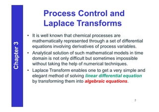
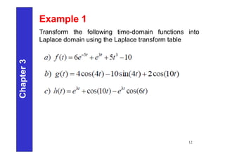
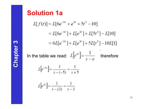
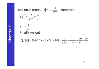
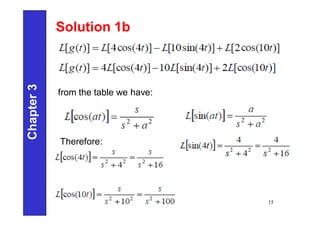
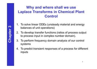
1. The document discusses Laplace transforms and their applications in solving differential equations that arise in mathematical models of chemical processes. 2. Laplace transforms allow the transformation of differential equations into algebraic equations, making them easier to solve. They can be used to solve linear ordinary differential equations (ODEs) that describe transient responses in unit operations. 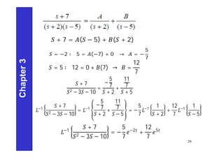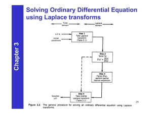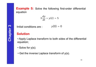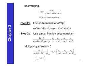3. The key steps in using Laplace transforms to solve ODEs are: taking the Laplace transform of the differential equation to obtain an algebraic equation relating the transform of the dependent variable to the independent variable and boundary conditions; solving for the transform of the dependent variable; and taking the inverse Laplace transform to find the original dependent variable as a function of time.

1. Chapter
3 CHEMICAL PROCESS OPTIMIZATION
AND CONTROL (CPO216B)
Laplace Transforms

2. Laplace Transforms
After learning this module you should be able:
• To define Laplace transform
• To convert mathematic expression in time domain t
to algebraic operations in complex numbers domain s
• To solve model equations in Laplace domain
Chapter
3
1

3. Process Control and
Laplace Transforms
• It is well known that chemical processes are
mathematically represented through a set of differential
equations involving derivatives of process variables.
• Analytical solution of such mathematical models in time
domain is not only difficult but sometimes impossible
without taking the help of numerical techniques.
• Laplace Transform enables one to get a very simple and
elegant method of solving linear differential equation
by transforming them into algebraic equations.
Chapter
3
2

4. Why and where shall we use
Laplace Transforms in Chemical Plant
Control
1. To solve linear ODEs (unsteady material and energy
balances of unit operations)
2. To develop transfer functions (ratios of process output
to process input in complex number domain).
3. To perform frequency domain analysis of our control
systems
4. To predict transient responses of a process for different
inputs
Chapter
3
3

5. Laplace Transforms - Definition
The above illustration of the Laplace transform is
regarded as an input function ƒ(t) which will be
transformed by the Laplace procedure (definite
integration of a certain product between 0 and ∞) to a
new output function F(s) which is now a function of a new
variable s, called the Laplace variable.
Chapter
3
4
Transformation
(integration)
ƒ(t) F(s)
input output

6. Laplace Transforms – Definition
(cont..)
Where
F(s) - the symbol for the Laplace transform
s - complex independent variable
ƒ(t) - some function of time to be transformed
L - an operator defined by the integral
Chapter
3
5
The Laplace transform of a function ƒ(t) is defined as
[ ( )] = −
. ( )
∞
0
= ( ) with s > 0

7. Laplace Transforms
Chapter
3
6
Constant function
For ƒ(t) = a (a constant)
[ ] = −
∞
0
= − [ − ]|0
∞
= 0 − − =

8. Laplace Transforms (cont..)
Chapter
3
7
Application: Consider a step function given by
ƒ(t) = K . u(t)
where K is a constant, u(t) is a step function given by
Therefore
u(t) = 1 t > 0
u(t) = 0 t ≤ 0
[ . ( )] = . ( ) −
∞
0
= −
∞
0
Since u(t) = 1 over the range of integration
Resulting [ . ( )] = − −
=0
=∞
= − (0 − 1) =
Laplace transform of a step function of magnitude K is
.
1

9. Useful properties of Laplace
Transforms
Chapter
3
8
• Linear operation:
[ ( )] = ( )
[ ( ) + ( )] = ( ) + ( )
• Laplace transform for power function:
• Laplace transform for exponential function:
[ ] =
!
+1
[ ] =
1
−
[ − ] =
1
+

10. Chapter
3
9
Useful properties of Laplace
Transforms (cont..)
• Laplace transform of derivatives
• Laplace transform for integration
• Laplace transform of a time delay function
( )
= ( ) − [ −1 (0) + −2 ′(0) + ⋯ + −2(0) + −1
(0)]
Where initial derivatives up to (n-1) are required
( ) =
1
[ ( )] =
1
( )
[ ( − )] = −
( )

11. Chpter
3
10
Table of Laplace transform
cos
sin

12. 11

13. Chapter
3
12
Example 1
Transform the following time-domain functions into
Laplace domain using the Laplace transform table

14. Chapter
3
13
Solution 1a
In the table we read: therefore

15. Chapter
3
14

16. Chapter
3
15
Solution 1b
from the table we have:
Therefore:

17. Chapter
3
16
Solution 1c
[ℎ( )]

18. Chapter
3
17
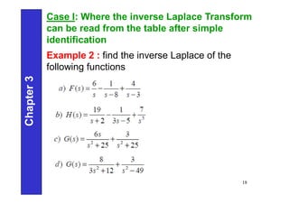
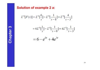
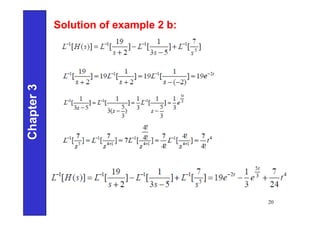
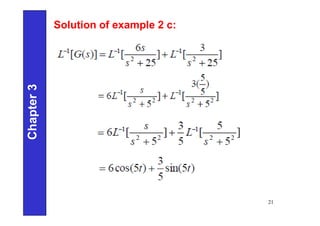
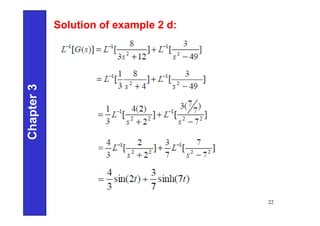
Inverse Laplace Transforms
• The inverse Laplace Transform transforms a function
from the Laplace domain into the time-domain.
−1[ ( )] = ( )
• For simple functions the inverse Laplace transform will
be directly read off a table by simple identification.
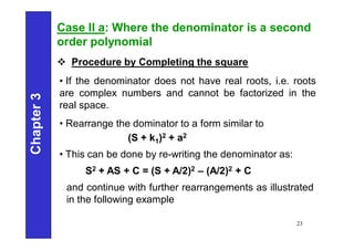
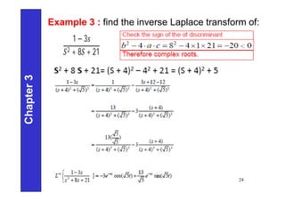
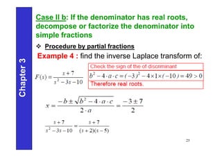
• Some functions will require to be rearranged into simple
functions in order to get their inverse from the table
• The inverse Laplace function is denoted as

19. Chapter
3
18
Case I: Where the inverse Laplace Transform
can be read from the table after simple
identification
Example 2 : find the inverse Laplace of the
following functions

20. Chapter
3
19
Solution of example 2 a:

21. Chapter
3
20
Solution of example 2 b:

22. Chapter
3
21
Solution of example 2 c:

23. Chapter
3
22
Solution of example 2 d:

24. Chapter
3
23
Case II a: Where the denominator is a second
order polynomial
 Procedure by Completing the square
• If the denominator does not have real roots, i.e. roots
are complex numbers and cannot be factorized in the
real space.
• Rearrange the dominator to a form similar to
(S + k1)2 + a2
• This can be done by re-writing the denominator as:
S2 + AS + C = (S + A/2)2 – (A/2)2 + C
and continue with further rearrangements as illustrated
in the following example

25. Chapter
3
24
Example 3 : find the inverse Laplace transform of:
1 − 3
2 + 8 +21

26. Chapter
3
25
Case II b: If the denominator has real roots,
decompose or factorize the denominator into
simple fractions
 Procedure by partial fractions
Example 4 : find the inverse Laplace transform of:

27. Chapter
3
26
+ 7 = ( − 5) + ( + 2)
= −2 ∶ 5 = (−7) + 0 → = −
5
7
= 5 ∶ 12 = 0 + (7) → =
12
7
+ 7
2 − 3 − 10
=
−
5
7
+ 2
+
11
7
+ 5
−1
+ 7
2 − 3 − 10
= −1
−
5
7
+ 2
+
11
7
− 5
= −
5
7
−1
1
+ 2
+
12
7
−1
1
− 5
−1
+ 7
2 − 3 − 10
= −
5
7
−2
+
12
7
5

28. Chapter
3
27
Case II c: Where the denominator is a
polynomial of higher order
 Decompose the denominator into simple fractions
The general procedure of decomposition into simple
fractions is given below:

29. Chapter
3
28
Example 5: Self Study – Evaluate the inverse Laplace
transform of the following functions.

30. Chapter
3
29
Solving Ordinary Differential Equation
using Laplace transforms

31. Chapter
3
30
Example 5: Solve the following first-order differential
equation
3 + ( ) = 5
Initial conditions are : (0) = 0
Solution
• Apply Laplace transform to both sides of the differential
equation;
• Get the inverse Laplace transform of y(s).
• Solve for y(s);

32. Chapter
3
31
From Laplace table

33. Example 6 (Ex 3.1 text book)
Solve the ODE
 
5 4 2 0 1 (3-26)
dy
y y
dt
  
First, take L of both sides of (3-26),
 
   
2
5 1 4
sY s Y s
s
  
Rearrange,
 
 
5 2
(3-34)
5 4
s
Y s
s s



Take inverse Laplace transform L-1,
 
 
1 5 2
5 4
s
y t
s s
  

  

 
L
From Table 3.1 we find solution y(t),
  0.8
0.5 0.5 (3-37)
t
y t e
 
Chapter
3
32

34. Example 2:
Example 2:
system at rest (steady state)
Step 1 Take L.T. (note zero initial conditions)
0
0
0
0
0
0
2
4
6
11
6 2
2
3
3
at t=
dt
du
)=
(
y
)=
(
y
)=
y(
u
dt
du
y
dt
dy
dt
y
d
dt
y
d









3 2
6 11 6 ( ) 4 2
s Y(s)+ s Y(s)+ sY(s) Y s = sU(s)+ U(s)

Chapter
3
To find transient response for u(t) = unit step at t > 0
1. Take Laplace Transform (L.T.)
2. Factor, use partial fraction decomposition
3. Take inverse L.T.
33

35. Rearranging,
Step 2a. Factor denominator of Y(s)
Step 2b. Use partial fraction decomposition
Multiply by s, set s = 0
input)
(
1
1
6
11
6
2
4
2
3
step
unit
s
U(s)
s
s
s
s
s+
Y(s)=





)
)(s+
)(s+
)=s(s+
s+
+
s
+
s(s 3
2
1
6
11
6 2
3
3
2
1
3
2
1
2
4 4
3
2
1







s
α
s
α
s
α
s
α
)
)(s+
)(s+
s(s+
s+
3
1
3
2
1
2
3
2
1
3
2
1
2
4
1
0
4
3
2
1
0



















α
s
α
s
α
s
α
s
α
)
)(s+
)(s+
(s+
s+
s
s
Chapter
3
34

36. For a2, multiply by (s+1), set s=-1 (same procedure
for a3, a4)
3
5
3
1 4
3
2 


 , α
, α
α
3
1
3
5
3
3
1 3
2





 


)
y(t
t
e
e
e
y(t)= t
t
t
Step 3. Take inverse of L.T.
You can use this method on any order of ODE,
limited only by factoring of denominator polynomial
(characteristic equation)
Must use modified procedure for repeated roots,
imaginary roots
Chapter
3
)
3
3
/
5
2
3
1
1
3
1
(






s
s
s
s
Y(s)=
35

37. END
Chapter
3
36