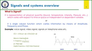
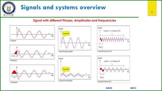
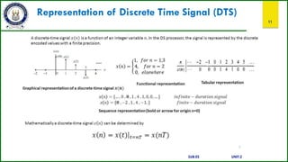
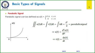
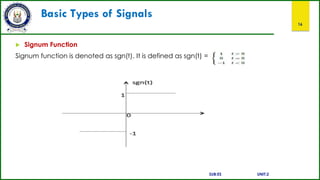
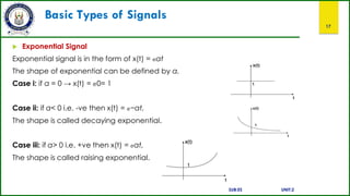
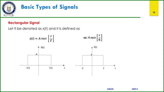
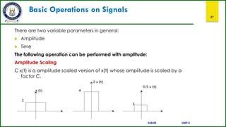
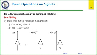
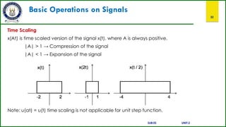
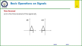
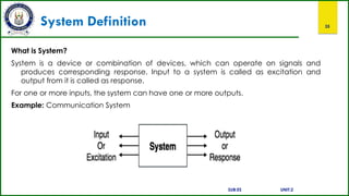
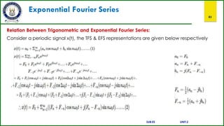
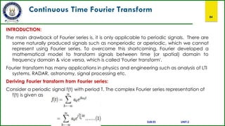
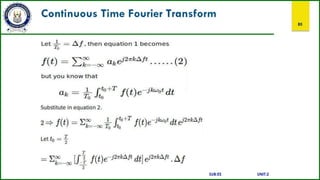
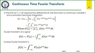
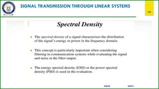
This document provides an overview of a course on signals and systems. It outlines the course outcomes which include explaining various signal and system types using Fourier series and transforms. It also describes analyzing signals through linear systems. The syllabus covers topics like Fourier series, continuous and discrete time Fourier transforms, Laplace and z-transforms, and signal transmission through linear systems. Basic signal types and signal classification are defined. Operations on signals like amplitude scaling and addition are also introduced.

![Classification of Systems
37
Linear and Non-linear Systems
A system is said to be linear when it satisfies superposition and homogenate principles. Consider two
systems with inputs as x1(t), x2(t), and outputs as y1(t), y2(t) respectively. Then, according to the
superposition and homogenate principles,
T [a1 x1(t) + a2 x2(t)] = a1 T[x1(t)] + a2 T[x2(t)]
∴ T [a1 x1(t) + a2 x2(t)] = a1 y1(t) + a2
y2(t)
From the above expression, is clear that response of overall system is equal to response of individual
system.
Example: y(t) = x2(t)
Solution:
y1 (t) = T[x1(t)] = x12(t)
y2 (t) = T[x2(t)] = x22(t)
T [a1 x1(t) + a2 x2(t)] = [ a1 x1(t) + a2 x2(t)]2
Which is not equal to a1 y1(t) + a2 y2(t). Hence the system is said to be non linear.
SUB:ES UNIT:2](https://image.slidesharecdn.com/sandsppt-221108045726-d1f4b7e3/85/s-and-s-ppt-pptx-37-320.jpg)
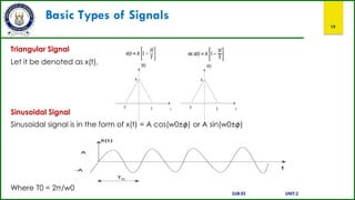
![Classification of Systems
38
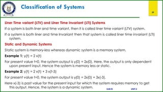
Time Variant and Time Invariant Systems
A system is said to be time variant if its input and output characteristics vary with time.
Otherwise, the system is considered as time invariant. The condition for time invariant system is:
y (n , t) = y(n-t)
The condition for time variant system is:
y (n , t) ≠ y(n-t)
Where y (n , t) = T[x(n-t)] = input change
y (n-t) = output change
Example:
y(n) = x(-n)
y(n, t) = T[x(n-t)] = x(-n-t)
y(n-t) = x(-(n-t)) = x(-n + t)
∴ y(n, t) ≠ y(n-t). Hence, the system is time
variant. SUB:ES UNIT:2](https://image.slidesharecdn.com/sandsppt-221108045726-d1f4b7e3/85/s-and-s-ppt-pptx-38-320.jpg)

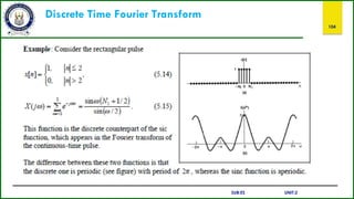
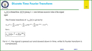
![Discrete Time Fourier Transform
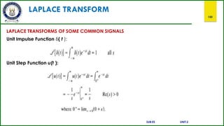
100
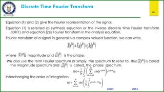
Discrete Time Fourier Transforms (DTFT)
Here we take the exponential signals to be where ‘w’is a real number. The
representation is motivated by the Harmonic analysis, but instead of following the
historical development of the representation we
defining equation.
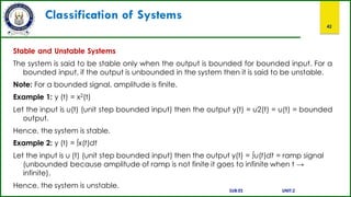
give directly the
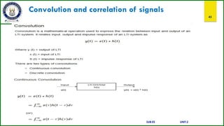
Let {x[n]} be discrete time signal such that
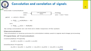
summable.
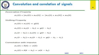
, that is sequence is absolutely
The sequence {x[n]} can be represented by a Fourier integral of the form,
Where,
SUB:ES UNIT:2](https://image.slidesharecdn.com/sandsppt-221108045726-d1f4b7e3/85/s-and-s-ppt-pptx-100-320.jpg)
![Discrete Time Fourier Transform
105
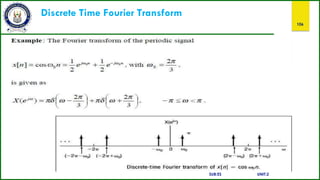
Fourier transform of Periodic Signals
For a periodic discrete-time signal,
its Fourier transform of this signal is periodic in w with period 2∏ , and is given
Now consider a periodic sequence x[n] with period N and with the Fourier series
representation
The Fourier transform is,
SUB:ES UNIT:2](https://image.slidesharecdn.com/sandsppt-221108045726-d1f4b7e3/85/s-and-s-ppt-pptx-105-320.jpg)
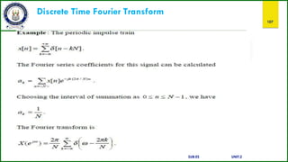
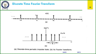
![Discrete Time Fourier Transform
109
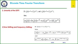
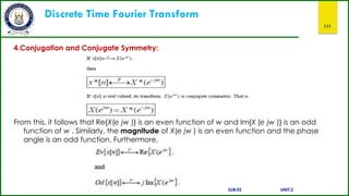
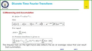
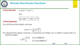
Properties of the Discrete Time Fourier Transform:
Let {x[n]}and {y[n]} be two signal, then their DTFT is denoted by and. The notation
is used to say that left hand side is the signal x[n] whose DTFT is given at right hand side.
1.Periodicity of the DTFT:
SUB:ES UNIT:2](https://image.slidesharecdn.com/sandsppt-221108045726-d1f4b7e3/85/s-and-s-ppt-pptx-109-320.jpg)
![Discrete Time Fourier Transform
115
8.Differentiation in Frequency
The right-hand side of the above equation is the Fourier transform of - jnx[n] . Therefore,
multiplying both sides by j , we see that
9.Parseval’s Relation
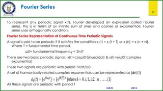
SUB:ES UNIT:2](https://image.slidesharecdn.com/sandsppt-221108045726-d1f4b7e3/85/s-and-s-ppt-pptx-115-320.jpg)
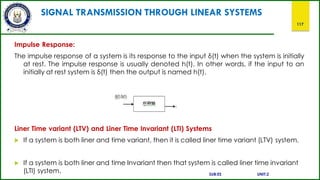
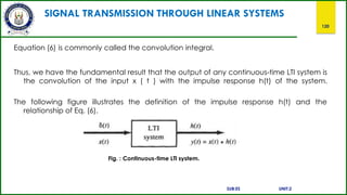
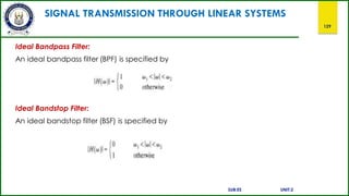
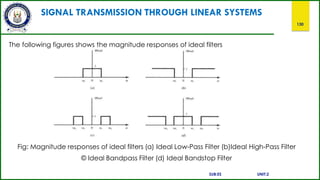
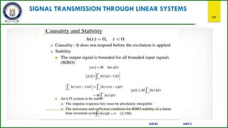
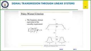
![SIGNAL TRANSMISSION THROUGH LINEAR SYSTEMS
116
Linear Systems:
A system is said to be linear when it satisfies superposition and homogenate principles. Consider two
systems with inputs as x1(t), x2(t), and outputs as y1(t), y2(t) respectively. Then, according to the
superposition and homogenate principles,
T [a1 x1(t) + a2 x2(t)] = a1 T[x1(t)] + a2 T[x2(t)]
∴ T [a1 x1(t) + a2 x2(t)] = a1 y1(t) + a2
y2(t)
From the above expression, is clear that response of overall system is equal to response of individual
system.
Example: y(t) = 2x(t)
Solution:
y1 (t) = T[x1(t)] = 2x1(t)
y2 (t) = T[x2(t)] = 2x2(t)
T [a1 x1(t) + a2 x2(t)] = 2[ a1 x1(t) + a2 x2(t)]
Which is equal to a1y1(t) + a2 y2(t). Hence the system is said to be UNIT:2](https://image.slidesharecdn.com/sandsppt-221108045726-d1f4b7e3/85/s-and-s-ppt-pptx-116-320.jpg)
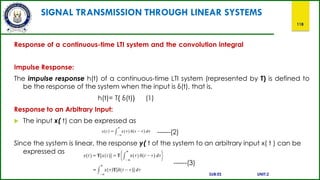
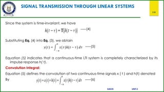
![SIGNAL TRANSMISSION THROUGH LINEAR SYSTEMS
123
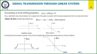
Distortion less transmission through a system:
Transmission is said to be distortion-less if the input and output have identical wave
shapes. i.e., in distortion-less transmission, the input x(t) and output y(t) satisfy the
condition:
y (t) = Kx(t - td)
Where td = delay time and
k = constant.
Take Fourier transform on both sides
FT[ y (t)] = FT[Kx(t - td)]
= K FT[x(t - td)]
SUB:ES UNIT:2](https://image.slidesharecdn.com/sandsppt-221108045726-d1f4b7e3/85/s-and-s-ppt-pptx-123-320.jpg)

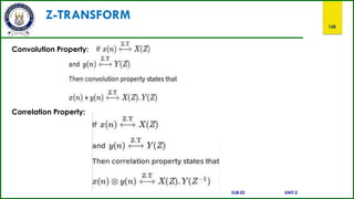

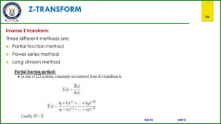
![Z-TRANSFORM
161
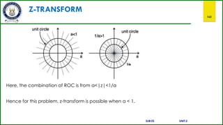
Example 1: Find z-transform and ROC of a n u[n]+a − n
u[−n−1] anu[n]+a−n
u[−n−1]
The plot of ROC has two conditions as a > 1 and a < 1, as we do not know a.
In this case, there is no combination ROC.
SUB:ES UNIT:2](https://image.slidesharecdn.com/sandsppt-221108045726-d1f4b7e3/85/s-and-s-ppt-pptx-161-320.jpg)
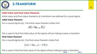
![Z-TRANSFORM
163
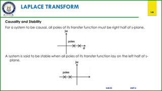
Causality and Stability
Causality condition for discrete time LTI systems is as follows:
A discrete time LTI system is causal when,
ROC is outside the outermost pole.
In The transfer function H[Z], the order of numerator cannot be grater than the order of
denominator.
Stability Condition for Discrete Time LTI Systems:
A discrete time LTI system is stable when
its system function H[Z] include unit circle |z|=1.
all poles of the transfer function lay inside the unit circle |z|=1.
SUB:ES UNIT:2](https://image.slidesharecdn.com/sandsppt-221108045726-d1f4b7e3/85/s-and-s-ppt-pptx-163-320.jpg)

![Z-TRANSFORM
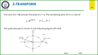
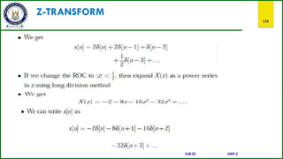
176
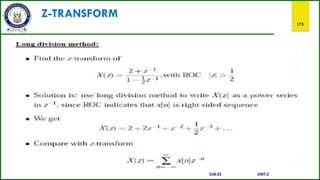
Example: A finite sequence x [ n ] is defined as
Find X(z) and its ROC.
Sol: We know that
For z not equal to zero or infinity, each term in X(z) will be finite and consequently X(z) will
converge. Note that X ( z ) includes both positive powers of z and negative powers of z.
Thus, from the result we conclude that the ROC of X ( z ) is 0 < lzl < m.
SUB:ES UNIT:2](https://image.slidesharecdn.com/sandsppt-221108045726-d1f4b7e3/85/s-and-s-ppt-pptx-176-320.jpg)
![Z-TRANSFORM
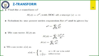
177
Example: Consider the sequence
Find X ( z ) and plot the poles and zeros of X(z).
Sol:
From the above equation we see that there is a pole of ( N - 1)th order at z = 0 and a pole at
z = a . Since x[n] is a finite sequence and is zero for n < 0, the ROC is IzI > 0. The N roots of
the numerator polynomial are at
SUB:ES UNIT:2](https://image.slidesharecdn.com/sandsppt-221108045726-d1f4b7e3/85/s-and-s-ppt-pptx-177-320.jpg)