Downloaded 318 times

(
2
1
)()]([1
*notes
Eq A
Eq B](https://image.slidesharecdn.com/laplacetransform-140421061347-phpapp01/85/Laplace-transform-2-320.jpg)
]([ =
The Laplace Transform of a unit step is:
s
1](https://image.slidesharecdn.com/laplacetransform-140421061347-phpapp01/85/Laplace-transform-4-320.jpg)

(
)]([ |0
as
tue at
+
⇔− 1
)(A transform
pair](https://image.slidesharecdn.com/laplacetransform-140421061347-phpapp01/85/Laplace-transform-9-320.jpg)
(
s
ttu ⇔
A transform
pair](https://image.slidesharecdn.com/laplacetransform-140421061347-phpapp01/85/Laplace-transform-10-320.jpg)
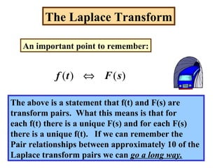
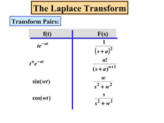
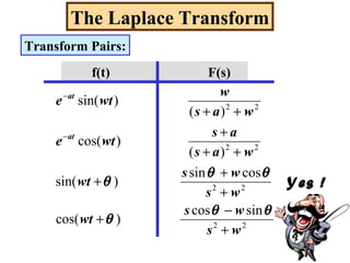
![The Laplace Transform
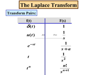
Building transform pairs:
22
0
11
2
1
2
)(
)][cos(
ws
s
jwsjws
dte
ee
wtL st
jwtjwt
+
=
+
−
−
=
+
= −
∞ −
∫
22
)()cos(
ws
s
tuwt
+
⇔ A transform
pair](https://image.slidesharecdn.com/laplacetransform-140421061347-phpapp01/85/Laplace-transform-11-320.jpg)
![The Laplace Transform
Time Shift
∫ ∫
∫
∞ ∞
−−+−
∞
−
=
∞→∞→→→
+==−=
−=−−
0 0
)(
)()(
,.,0,
,
)()]()([
dxexfedxexf
SoxtasandxatAs
axtanddtdxthenatxLet
eatfatuatfL
sxasaxs
a
st
)()]()([ sFeatuatfL as−
=−−](https://image.slidesharecdn.com/laplacetransform-140421061347-phpapp01/85/Laplace-transform-12-320.jpg)
]([
asFdtetf
dtetfetfeL
tas
statat
)()]([ asFtfeL at
+=−](https://image.slidesharecdn.com/laplacetransform-140421061347-phpapp01/85/Laplace-transform-13-320.jpg)
![The Laplace Transform
Example: Using Frequency Shift
Find the L[e-at
cos(wt)]
In this case, f(t) = cos(wt) so,
22
22
)(
)(
)(
)(
was
as
asFand
ws
s
sF
++
+
=+
+
=
22
)()(
)(
)]cos([
was
as
wteL at
++
+
=−](https://image.slidesharecdn.com/laplacetransform-140421061347-phpapp01/85/Laplace-transform-14-320.jpg)

![The Laplace Transform
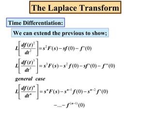
Time Differentiation:
If the L[f(t)] = F(s), we want to show:
)0()(]
)(
[ fssF
dt
tdf
L −=
Integrate by parts:
)(),(
)(
,
tfvsotdfdt
dt
tdf
dv
anddtsedueu stst
===
−== −−
*note](https://image.slidesharecdn.com/laplacetransform-140421061347-phpapp01/85/Laplace-transform-17-320.jpg)
![The Laplace Transform
Time Differentiation:
Making the previous substitutions gives,
[ ]
∫
∫
∞
−
∞
−∞−
+−=
−−=
0
0
0
)()0(0
)()( |
dtetfsf
dtsetfetf
dt
df
L
st
stst
So we have shown:
)0()(
)(
fssF
dt
tdf
L −=
](https://image.slidesharecdn.com/laplacetransform-140421061347-phpapp01/85/Laplace-transform-18-320.jpg)
![The Laplace Transform
Final Value Theorem:Example:
Given:
[ ] ttesFnote
s
s
sF t
3cos)(
3)2(
3)2(
)( 21
22
22
−
=
++
−+
= −
Find )(∞f .
[ ] 0
3)2(
3)2(
lim)(lim)( 22
22
=
++
−+
==∞
s
s
sssFf
0→s0→s](https://image.slidesharecdn.com/laplacetransform-140421061347-phpapp01/85/Laplace-transform-29-320.jpg)


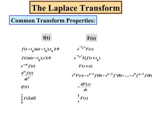
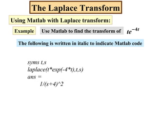
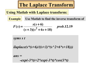
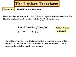
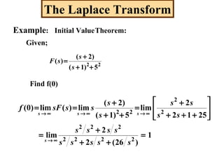
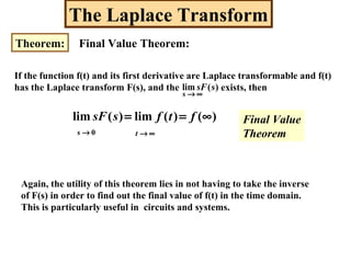
The document provides an overview of the Laplace transform including: - Definitions of the Laplace transform and inverse Laplace transform - Transform pairs for common functions like unit step, unit impulse, exponentials, sinusoids - Properties for time shifting, frequency shifting, differentiation, integration - Theorems for finding the initial value and final value of a function from its Laplace transform - Examples of using the Laplace transform and its properties


