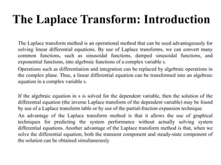
The Laplace Transform:Introduction
The Laplace transform method is an operational method that can be used advantageously for
solving linear differential equations. By use of Laplace transforms, we can convert many
common functions, such as sinusoidal functions, damped sinusoidal functions, and
exponential functions, into algebraic functions of a complex variable s.
Operations such as differentiation and integration can be replaced by algebraic operations in
the complex plane. Thus, a linear differential equation can be transformed into an algebraic
equation in a complex variable s.
If the algebraic equation in s is solved for the dependent variable, then the solution of the
differential equation (the inverse Laplace transform of the dependent variable) may be found
by use of a Laplace transform table or by use of the partial-fraction expansion technique.
An advantage of the Laplace transform method is that it allows the use of graphical
techniques for predicting the system performance without actually solving system
differential equations. Another advantage of the Laplace transform method is that, when we
solve the differential equation, both the transient component and steady-state component of
the solution can be obtained simultaneously
3.
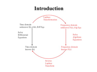
Introduction
Tim e domain
unknow n f(t), d/dt, D iff Eqs
Frequency dom ain
unknow n F(s), A lg Eqs
Laplace
Transform ation
Solve
A lgebraic
Equations
Frequency dom ain
know n F(s)
Tim e dom ain
know n f(t)
Solve
D ifferential
Equations
Inverse
Laplace
Transform
4.
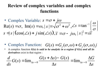
Review of complexvariables and complex
functions
• Complex Variable:
• Complex Function:
• A complex function G(s) is said to be analytic in a region if G(s) and all its
derivatives exist in that region :
s j
Re( ) ,
s
Im( ) ,
s
2 2
| | ,
s
1
tan
s
| | cos( ) sin( ) ,
s s s j s
,
s j
2
| |
s ss
( ) ( , ) ( , )
x y
G s G G j
0 0
( ) ( )
( ) lim lim
s s
d G s s G s G
G s
ds s s
5.
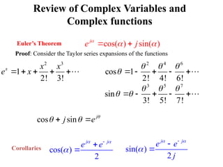
Review of ComplexVariables and
Complex functions
Euler’s Theorem cos( ) sin( )
j
e j
Corollaries cos( )
2
j j
e e
sin( )
2
j j
e e
j
Proof: Consider the Taylor series expansions of the functions
2 3
1
2! 3!
x x x
e x
2 4 6
cos 1
2! 4! 6!
3 5 7
sin
3! 5! 7!
cos sin j
j e
6.
Laplace Transformation
• Letus define:
– f(t)= a function of time t such that f ( t ) = 0 for t < 0
– s = a complex variable
– = an operational symbol indicating that the
quantity that it prefixes is to be transformed by the
Laplace integral
– F(s) = Laplace transform of f( t )
Then the Laplace Transform of f(t) is:
L
0
( ) st
e d
f t t
0
[ ] (
) ( )
)
( st
f t f
F t
s e dt
L
7.
Laplace Transform Theorems
1.Linearity:
2. Superposition:
3. Translation in time:
4. Complex differentiation:
5. Translation in the s Domain:
6. Real Differentiation:
7. Real Integration:
8. Final Value:
9. Initial Value:
10.Complex Integration:
[ ] [
( ) ( )] ( )
f t f t F s
L L
1
1 2
1 2 2
[ ] [ ]
( ) [ ] ( ) ( )
( ) ( ) ( )
f t f t f t t F s F s
f
L L L
1
( ) (
[ ] ( )
) s
f t u e F
t s
L
[ ] ( )
( )
d
F s
tf
ds
t
L
( )
[ ] ( )
t
e t s
f F
L
[ ] ( ) (
( ) 0 )
sF s f
Df t
L
1
1
0
( )
( ) )
(0
[ ]
(0
)
t
F s D f
s
f t dt f
s
D
L
0
lim ( ) lim ( )
s t
sF s f t
0
lim ( ) lim ( )
s t
sF s f t
[ ]
(
)
)
(
F
f
d
t
s
t
s
L
8.
Derivation of LaplaceTransforms of Simple
Functions
• Step Function
(Echelon Unite):
• Exponential Function:
0
[1(
0, 0
1( ) ]
) ( )
0
1
,
1,
t
st
t
e d
t
t
t
t
t
t
L
0 0
1( ) 1( )
[ ]
t t
st st
t t
e
t t dt e dt
L
0
1
t
st
t
e
s
1
s
0, 0
( )
, 0
at
t
f t
Ae t
0
[ ]
a t
t at s A
e dt
Ae A
s a
e
L
9.
Derivation of LaplaceTransforms of Simple
Functions
• Ramp Function:
• Sinusoidal Function:
0, 0
( )
, 0
t
f t
At t
0 0
0
2
0
)
[ ]
st st
st
st
e Ae
e dt At dt
s s
A A
At A
e d
s s
t
t
L
0, 0
( )
sin , 0
t
f t
A wt t
0
2 2
2
1 1
2 2
sin ( ) st
j t j t
A
e dt
j
A A Aw
j s jw j
A wt
s jw s w
e e
L
10.
Inverse Laplace Transformation
Theinverse Laplace transform can be obtained by use of the inversion integral
given by:
• Partial-Fraction Expansion Method for Finding Inverse Laplace
Transforms:
For problems in control systems analysis, F(s), the Laplace transform off (t),
frequently occurs in the form:
where A(s) and B(s) are polynomials in s. In the expansion of F(s) = B(s)/A(s)
into a partial-fraction form, it is important that the highest power of s in A(s)
be greater than the highest power of s in B(s).
If F(s) is broken up into components:
-1 1
[ ] (
( ) ( )
2
)
c j
st
c j
f t F s e ds
j
F s
L
( ) ( ) / ( )
F s B s A s
1 2
( ) ( ) ( ) ( )
n
F s F s F s F s
1 2
-1 -1 -1 -1
( ) ( ) ( ) ( )
[ ] [ ] [ ] [ ]
n
F s F s F s F s
L L L L
11.
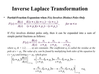
Inverse Laplace Transformation
•Partial-Fraction Expansion when F(s) Involves Distinct Poles Only
If F(s) involves distinct poles only, then it can be expanded into a sum of
simple partial fractions as follows:
where ak (k = 1,2,. . . , n) are constants. The coefficient ak is called the residue at the
pole at s = -pk. The value of a, can be found by multiplying both sides of the equation by
( s + pk) and letting s = -pk, which gives
1 2
1 2
( )( ) ( )
( )
( ) ,
( ) ( )( ) ( )
m
n
K s z s z s z
B s
F s for m n
A s s p s p s p
1 2
1 2
( )
( )
( )
n
n
a
a a
B s
F s
A s s p s p s p
1 2
1 2
( )
( ) k
k
k k k
s p
k n
k k k
k n s p
a a
B s
s p s p s p
A s s p s p
a a
s p s p a
s p s p
12.
Inverse Laplace Transformation
•Example:
The partial-fraction expansion of F(s) is:
3
( )
( 1)( 2)
s
F s
s s
3
( )
( 1)( 2) 1 2
s
F s
s s s s
B
A
1
1
3 3
( 1) 2
( 1)( 2) 2 s
s
s s
A s
s s s
2
2
3 3
( 2) 1
( 1)( 2) 1 s
s
s s
B s
s s s
Thus -1 -1 -1
2
2 1
( ) [ ]
(
2
2
)
1
t t
f t
s s
e e
F s
L L L
13.
Inverse Laplace Transformation
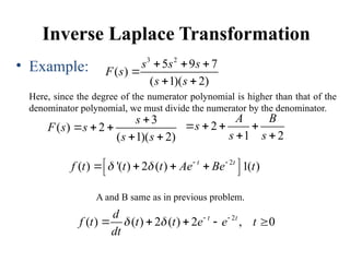
•Example:
Here, since the degree of the numerator polynomial is higher than that of the
denominator polynomial, we must divide the numerator by the denominator.
3 2
5 9 7
( )
( 1)( 2)
s s s
F s
s s
3
( ) 2
( 1)( 2)
s
F s s
s s
2
1 2
A B
s
s s
2
( ) '( ) 2 ( ) 1( )
t t
f t t t Ae Be t
2
( ) ( ) 2 ( ) 2 , 0
t t
d
f t t t e e t
dt
A and B same as in previous problem.
14.
Inverse Laplace Transformation
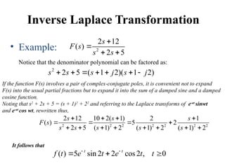
•Example:
Notice that the denominator polynomial can be factored as:
2
2 12
( )
2 5
s
F s
s s
2
2 5 ( 1 2)( 1 2)
s s s j s j
If the function F(s) involves a pair of complex-conjugate poles, it is convenient not to expand
F(s) into the usual partial fractions but to expand it into the sum of a damped sine and a damped
cosine function.
Noting that s2
+ 2s + 5 = (s + 1)2
+ 22
and referring to the Laplace transforms of e-at
sinwt
and e-at
cos wt, rewritten thus,
2 2 2 2 2 2 2
2 12 10 2( 1) 2 1
( ) 5 2
2 5 ( 1) 2 ( 1) 2 ( 1) 2
s s s
F s
s s s s s
It follows that
( ) 5 sin 2 2 cos2 , 0
t t
f t e t e t t
15.
Inverse Laplace Transformation
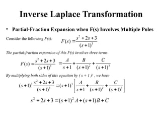
•Partial-Fraction Expansion when F(s) Involves Multiple Poles
Consider the following F(s):
2
3
2 3
( )
( 1)
s s
F s
s
The partial-fraction expansion of this F(s) involves three terms
2
3
2 3
( )
( 1)
s s
F s
s
2 3
1 ( 1) ( 1)
A B C
s s s
By multiplying both sides of this equation by ( s + 1 )3
, we have
2
3 3
3 2 3
2 3
( 1) ( 1)
( 1) 1 ( 1) ( 1)
s s A B C
s s
s s s s
2 2
2 3 ( 1) ( 1)
s s s A s B C
16.
Inverse Laplace Transformation
2
1
1
2 3 2 2 0
s
s
d
B s s s
ds
2
3 3
3 2 3
1
1
2 3
( 1) ( 1) 2
( 1) 1 ( 1) ( 1) s
s
s s A B C
s s C
s s s s
Then letting s = -1
2
2
2
1
2 3
s
d
A s s
ds
2
1
2 2
s
d
s
ds
2
2 2
( ) 2
2
t t t t t
C
f t Ae Bte t e e t e
Thus
17.
Solving Linear, Time-Invariant,Differential
Equations
In this section we are concerned with the use of the Laplace transform
method in solving linear, time-invariant, differential equations.
• The Laplace transform method yields the complete solution
(complementary solution and particular solution) of linear, time-invariant,
differential equations. Classical methods for finding the complete solution
of a differential equation require the evaluation of the integration
constants from the initial conditions. In the case of the Laplace transform
method, however, this requirement is unnecessary because the initial
conditions are automatically included in the Laplace transform of the
differential equation.
• If all initial conditions are zero, then the Laplace transform of the
differential equation is obtained simply by replacing d/ dt with s, d2
/ dt2
with s2
, and so on.
• In solving linear, time-invariant, differential equations by the Laplace
transform method, two steps are involved:
18.
Solving Linear, Time-Invariant,Differential
Equations
1. By taking the Laplace transform of each term in
the given differential equation, convert the
differential equation into an algebraic equation
in s and obtain the expression for the Laplace
transform of the dependent variable by
rearranging the algebraic equation.
2. The time solution of the differential equation is
obtained by finding the inverse Laplace
transform of the dependent variable.
19.
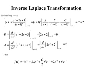
Solving Linear, Time-Invariant,Differential
Equations
Example: Find the solution x(t) of the differential equation
3 2 0, (0) ,
x x x x a x b
By writing the Laplace transform of x(t) as X(s), we obtain:
2
[ ] ( ) (0)
[ ] ( ) (0) (0)
x
x
sX s x
s X s sx x
L
L
And so the given differential equation becomes
2
( ) (0) (0) 3 ( ) (0) 2 ( ) 0
s X s sx x sX s x X s
By substituting the given initial conditions into this last equation, we obtain
2
3 2 ( ) 3
s s X s sa b a
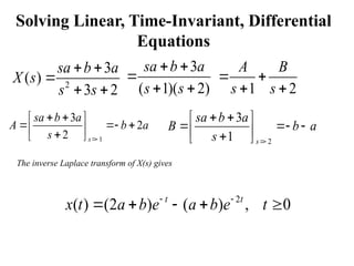
20.
Solving Linear, Time-Invariant,Differential
Equations
2
3
( )
3 2
sa b a
X s
s s
3
( 1)( 2)
sa b a
s s
The inverse Laplace transform of X(s) gives
1 2
A B
s s
1
3
2
2 s
sa b a
A b a
s
2
3
1 s
sa b a
B b a
s
2
( ) (2 ) ( ) , 0
t t
x t a b e a b e t
Editor's Notes
#4 Before we present the Laplace transformation, we shall review the complex variable and complex function.
A complex number has a real part and an imaginary part, both of which are constant.
A complex function G(s),a function of s, has a real part and an imaginary part or where Gx and Gy, are real quantities. The magnitude of G(s) is sqrt(Gx^2+Gy^2) and the angle of G(s) is t a n - ' ( Gy /Gx) the angle is measured counterclockwise from the positive real axis. The complex conjugate of G(s) is G(s) = Gx - jGy.
The derivative of an analytic function G(s) is given by:
#5 Since As = Aa + jAw, As can approach zero along an infinite number of different paths. It can be shown, but is stated without a proof here, that if the derivatives taken along two particular paths, that is, As = Au and As = jAw, are equal, then the derivative is unique for any other path As = A a + jAw and so the derivative exists.
For a particular path As = Au (which means that the path is parallel to the real axis).
For another particular path As = jAw (which means that the path is parallel to the imaginary axis).
#7 As an example, consider the following G(s):
It can be seen that, except at s = -1 (that is, a = -1, w = 0), G(s) satisfies the Cauchy-Riemann conditions:
Hence G(s) = l/(s + 1) is analytic in the entire s plane except at s = -1.The derivative dG (s)/ ds, except at s = 1, is found to be:
Note that the derivative of an analytic function can be obtained simply by differentiating G(s) with respect to s.
#10 We shall first present a definition of the Laplace transformation and a brief discussion of the condition for the existence of the Laplace transform and then provide examples for illustrating the derivation of Laplace transforms of several common functions.
#11 Several theorems that are useful in applying the Laplace transform are presented in this section. In general, they are helpful in evaluating transforms:
Theorem 1: Linearity. If a is a constant or is independent of s and t, and if f (t) is transformable, then
Theorem 2: Superposition. If f1(t) and f2(t) are both Laplace-transformable, the principle of superposition applies
Theorem 3: Translation in time. If the Laplace transform of f (t) is F(s) and a is a positive real number, the Laplace transform of the translated function f (t-a)u1(t-a) is
Theorem 4: Complex differentiation. If the Laplace transformof f (t) is F(s), then:
Multiplication by time in the real domain entails differentiation with respect to s in the s domain.
Theorem 5: Translation in the s Domain. If the Laplace transform of f (t) is F(s) and a is either real or complex, then
Multiplication of eat in the real domain becomes translation in the s domain
Theorem 6: Real Differentiation. If theLaplace transformof f (t) isF(s),and if the first derivative of f (t) with respect to time Df (t) is transformable, then
The term f (0+) is the value of the right-hand limit of the function f (t) as the origin t(0+) is approached from the right side (thus through positive
values of time). This includes functions, such as the step function, that may be undefined at t0+. For simplicity, the plus sign following the zero is usually omitted, although its presence is implied.
Theorem 7: Real Integration. If the Laplace transform of f (t) is F(s), its integral is transformable and the value of its transform is:
The term D1 f (0+) is the constant of integration and is equal to the value of the integral as the origin is approached from the positive or right side.
Theorem 8: Final Value. If f (t) and Df (t) are Laplace transformable, if the Laplace transformof f (t) is F(s), and if the limit f (t) as t infinit exists,then:
This theorem states that the behavior of f (t) in the neighborhood of t=infinit related to the behavior of sF(s) in the neighborhood of s=0. If sF(s) has poles [values of s for which jsF(s)j becomes infinite] on the imaginary axis (excluding the origin) or in the right-half s plane, there is no finite final value of f (t) and the theorem cannot be used. If f (t) is sinusoidal, the theorem is invalid, since L(sin wt) has poles at s=jw and limt t infinit
sinwt does not exist. However, for poles of sF(s) at the origin, s=0, this theorem gives the final value of f(inifint)=inifinit. This correctly describes the behavior of f (t) as t inifinit.
Theorem 9: Initial Value. If the function f (t) and its first derivative are Laplace transformable, if the Laplace transform of f (t) is F(s), and if
Lim s infinit sF(s) exists, then
This theoremstates that the behavior of f (t) in the neighborhood of t=0 is related to the behavior of sF(s) in the neighborhood of s=infinit.There are no limitations on the locations of the poles of sF(s).
Theorem 10: Complex Integration. If the Laplace transform of f (t) is F(s) and if f (t)/t has a limit as t inifinit, then
#14 where c, the abscissa of convergence, is a real constant and is chosen larger than the real parts of all singular points of F(s).
However, the inversion integral is complicated and, therefore, its use is not recommended for finding inverse Laplace transforms of commonly encountered functions in control engineering.
A convenient method for obtaining inverse Laplace transforms is to use a table of Laplace transforms. In this case, the Laplace transform must be in a form immediately recognizable in such a table. Quite often the function in question may not appear in tables of Laplace transforms available to the engineer. If a particular transform F(s) cannot be found in a table, then we may expand it into partial fractions and write F(s) in terms of simple
If such is not the case, the numerator B(s) must be divided by the denominator A(s) in order to produce a polynomial in s plus a remainder (a ratio of polynomials in s whose numerator is of lower degree than the denominator).
#15 Consider F ( s ) written in the factored form:
where p1 p2 . . . , pn and z1,, z2,. . . , zm, are either real or complex quantities, but for each complex pi or zi, there will occur the complex conjugate of p, or z,, respectively
We see that all the expanded terms drop out with the exception of ak. Thus the residue ak is found from
#17 Note that the Laplace transform of the unit-impulse function S(t) is 1 and that the Laplace transform of dS(t)/ dt is s.
![Laplace Transformation
• Let us define:
– f(t)= a function of time t such that f ( t ) = 0 for t < 0
– s = a complex variable
– = an operational symbol indicating that the
quantity that it prefixes is to be transformed by the
Laplace integral
– F(s) = Laplace transform of f( t )
Then the Laplace Transform of f(t) is:
L
0
( ) st
e d
f t t
0
[ ] (
) ( )
)
( st
f t f
F t
s e dt
L](https://image.slidesharecdn.com/laplacetransformlinear-250322130032-8be74e15/85/Laplace-tranbeereerrhhhsform-linear-pptx-6-320.jpg)
![Laplace Transform Theorems
1. Linearity:
2. Superposition:
3. Translation in time:
4. Complex differentiation:
5. Translation in the s Domain:
6. Real Differentiation:
7. Real Integration:
8. Final Value:
9. Initial Value:
10.Complex Integration:
[ ] [
( ) ( )] ( )
f t f t F s
L L
1
1 2
1 2 2
[ ] [ ]
( ) [ ] ( ) ( )
( ) ( ) ( )
f t f t f t t F s F s
f
L L L
1
( ) (
[ ] ( )
) s
f t u e F
t s
L
[ ] ( )
( )
d
F s
tf
ds
t
L
( )
[ ] ( )
t
e t s
f F
L
[ ] ( ) (
( ) 0 )
sF s f
Df t
L
1
1
0
( )
( ) )
(0
[ ]
(0
)
t
F s D f
s
f t dt f
s
D
L
0
lim ( ) lim ( )
s t
sF s f t
0
lim ( ) lim ( )
s t
sF s f t
[ ]
(
)
)
(
F
f
d
t
s
t
s
L](https://image.slidesharecdn.com/laplacetransformlinear-250322130032-8be74e15/85/Laplace-tranbeereerrhhhsform-linear-pptx-7-320.jpg)
![Derivation of Laplace Transforms of Simple
Functions
• Step Function
(Echelon Unite):
• Exponential Function:
0
[1(
0, 0
1( ) ]
) ( )
0
1
,
1,
t
st
t
e d
t
t
t
t
t
t
L
0 0
1( ) 1( )
[ ]
t t
st st
t t
e
t t dt e dt
L
0
1
t
st
t
e
s
1
s
0, 0
( )
, 0
at
t
f t
Ae t
0
[ ]
a t
t at s A
e dt
Ae A
s a
e
L](https://image.slidesharecdn.com/laplacetransformlinear-250322130032-8be74e15/85/Laplace-tranbeereerrhhhsform-linear-pptx-8-320.jpg)
![Derivation of Laplace Transforms of Simple
Functions
• Ramp Function:
• Sinusoidal Function:
0, 0
( )
, 0
t
f t
At t
0 0
0
2
0
)
[ ]
st st
st
st
e Ae
e dt At dt
s s
A A
At A
e d
s s
t
t
L
0, 0
( )
sin , 0
t
f t
A wt t
0
2 2
2
1 1
2 2
sin ( ) st
j t j t
A
e dt
j
A A Aw
j s jw j
A wt
s jw s w
e e
L](https://image.slidesharecdn.com/laplacetransformlinear-250322130032-8be74e15/85/Laplace-tranbeereerrhhhsform-linear-pptx-9-320.jpg)
![Inverse Laplace Transformation
The inverse Laplace transform can be obtained by use of the inversion integral
given by:
• Partial-Fraction Expansion Method for Finding Inverse Laplace
Transforms:
For problems in control systems analysis, F(s), the Laplace transform off (t),
frequently occurs in the form:
where A(s) and B(s) are polynomials in s. In the expansion of F(s) = B(s)/A(s)
into a partial-fraction form, it is important that the highest power of s in A(s)
be greater than the highest power of s in B(s).
If F(s) is broken up into components:
-1 1
[ ] (
( ) ( )
2
)
c j
st
c j
f t F s e ds
j
F s
L
( ) ( ) / ( )
F s B s A s
1 2
( ) ( ) ( ) ( )
n
F s F s F s F s
1 2
-1 -1 -1 -1
( ) ( ) ( ) ( )
[ ] [ ] [ ] [ ]
n
F s F s F s F s
L L L L](https://image.slidesharecdn.com/laplacetransformlinear-250322130032-8be74e15/85/Laplace-tranbeereerrhhhsform-linear-pptx-10-320.jpg)
![Inverse Laplace Transformation
• Example:
The partial-fraction expansion of F(s) is:
3
( )
( 1)( 2)
s
F s
s s
3
( )
( 1)( 2) 1 2
s
F s
s s s s
B
A
1
1
3 3
( 1) 2
( 1)( 2) 2 s
s
s s
A s
s s s
2
2
3 3
( 2) 1
( 1)( 2) 1 s
s
s s
B s
s s s
Thus -1 -1 -1
2
2 1
( ) [ ]
(
2
2
)
1
t t
f t
s s
e e
F s
L L L](https://image.slidesharecdn.com/laplacetransformlinear-250322130032-8be74e15/85/Laplace-tranbeereerrhhhsform-linear-pptx-12-320.jpg)
![Solving Linear, Time-Invariant, Differential
Equations
Example: Find the solution x(t) of the differential equation
3 2 0, (0) ,
x x x x a x b
By writing the Laplace transform of x(t) as X(s), we obtain:
2
[ ] ( ) (0)
[ ] ( ) (0) (0)
x
x
sX s x
s X s sx x
L
L
And so the given differential equation becomes
2
( ) (0) (0) 3 ( ) (0) 2 ( ) 0
s X s sx x sX s x X s
By substituting the given initial conditions into this last equation, we obtain
2
3 2 ( ) 3
s s X s sa b a
](https://image.slidesharecdn.com/laplacetransformlinear-250322130032-8be74e15/85/Laplace-tranbeereerrhhhsform-linear-pptx-19-320.jpg)