The Fourier transform decomposes a signal into its constituent frequencies. The document provides definitions and properties of the Fourier transform including:
- The Fourier transform of a signal exists if the signal is integrable.
- The inverse Fourier transform retrieves the original signal from its frequency spectrum.
- Properties include linearity, time shifting which changes the phase but not amplitude spectrum, time scaling which scales the frequency axis, and duality which relates a signal and its frequency spectrum.
- Examples demonstrate calculating the Fourier transform of simple signals like a rectangular pulse.


![4
Fourier Transform
Determine the Fourier transform of the Delta function δ(t)
Example
0
( ) ( ) 1
j t j
X t e dt e
ω ω
ω δ
∞
− −
−∞
= = =
∫
1
X(ω)
ω
Fourier Transform
Properties of the Fourier Transform
We summarize several important properties of the Fourier Transform as follows.
1. Linearity (Superposition)
1 1
( ) ( )
x t X ω
⇔ 2 2
( ) ( )
x t X ω
⇔
1 1 2 2 1 1 2 2
( ) ( ) ( ) ( )
a x t a x t a X a X
ω ω
+ ⇔ +
Then,
If and
Proof:
[ ]
1 1 2 2 1 1 2 2
1 1 2 2
( ) ( ) ( ) ( )
( ) ( )
j t j t j t
a x t a x t e dt a x t e dt a x t e dt
a X a X
ω ω ω
ω ω
∞ ∞ ∞
− − −
−∞ −∞ −∞
+ = +
= +
∫ ∫ ∫](https://image.slidesharecdn.com/fouriertransform-220125153301/85/Fourier-transform-4-320.jpg)


![10
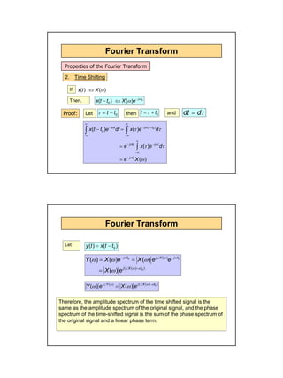
Fourier Transform
Determine the Fourier transform of and
Example: cos ct
ω sin ct
ω
[ ]
1 1
( ) cos ( ) ( ) ( )
2 2
c c
j t j t
c c c
x t t e e X
ω ω
ω ω π δ ω ω δ ω ω
−
= = + ⇔ = − + +
[ ]
1 1 1
( ) cos ( ) ( ) ( )
2 2 2
c c
j t j t
c c c
x t t e e X f f f f f
ω ω
ω δ δ
−
= = + ⇔ = − + +
or
f
1/2
fc
-fc
The phase spectrum is zero everywhere.
X(f)
Fourier Transform
[ ]
1 1
( ) sin ( ) ( ) ( )
2 2
c c
j t j t
c c c
x t t e e X j
j j
ω ω
ω ω π δ ω ω δ ω ω
−
= = − ⇔ = − − − +
[ ]
1 1
( ) sin ( ) ( ) ( )
2 2 2
c c
j t j t
c c c
j
x t t e e X f f f f f
j j
ω ω
ω δ δ
− −
= = − ⇔ = − − +
f
π/2
-fc
fc
-π/2
f
1/2
fc
-fc
|X(f)|
θ(f)](https://image.slidesharecdn.com/fouriertransform-220125153301/85/Fourier-transform-10-320.jpg)
![11
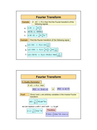
Fourier Transform
7. Modulation
If then
Proof:
( ) ( )
x t X ω
⇔
[ ]
1
( )cos( ) ( ) ( )
2
c c c
x t t X X
ω ω ω ω ω
⇔ − + +
[ ]
( ) ( )
1
( )cos( ) ( )
2
1
( ) ( )
2
1
( ) ( )
2
c c
c c
j t j t
j t j t
c
j t j t
c c
x t t e dt x t e e e dt
x t e dt x t e dt
X X
ω ω
ω ω
ω ω ω ω
ω
ω ω ω ω
∞ ∞
− −
−∞ −∞
∞ ∞
− − − +
−∞ −∞
= +
= +
= − + +
∫ ∫
∫ ∫
Fourier Transform
8. Time Differentiation:
If then
Proof:
( ) ( )
x t X ω
⇔
( )
( )
dx t
j X
dt
ω ω
⇔
( )
( ) ( )
n
n
n
d x t
j X
dt
ω ω
⇔
General case
Taking the derivative of the inverse Fourier transform
1
( ) ( )
2
j t
x t X e d
ω
ω ω
π
∞
−∞
= ∫
( ) 1
( )
2
j t
dx t
j X e d
dt
ω
ω ω ω
π
∞
−∞
= ∫
( )
( )
dx t
j X
dt
ω ω
⇔
we obtain
Therefore](https://image.slidesharecdn.com/fouriertransform-220125153301/85/Fourier-transform-11-320.jpg)


![Digital Signal Processing[ECEG-3171]-Ch1_L03](https://cdn.slidesharecdn.com/ss_thumbnails/dspl3-180427094423-thumbnail.jpg?width=640&height=640&fit=bounds)