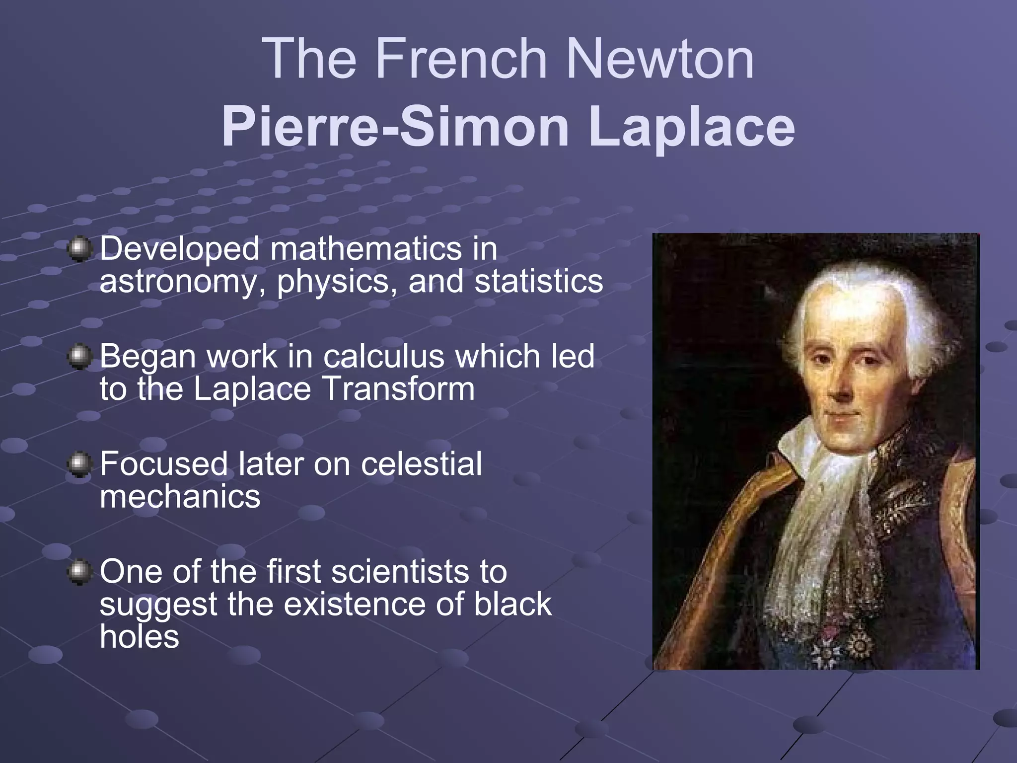
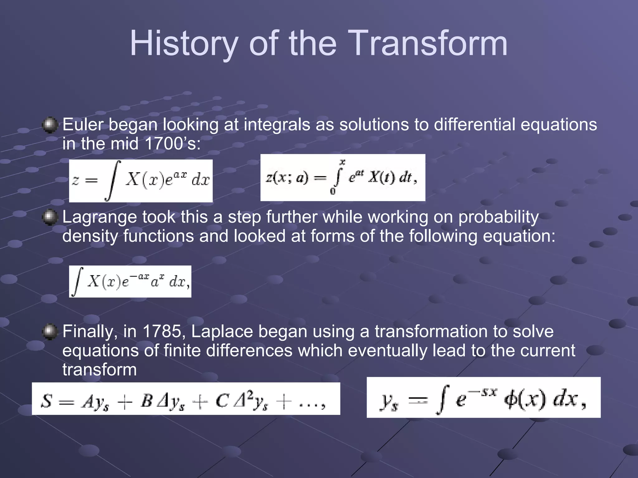
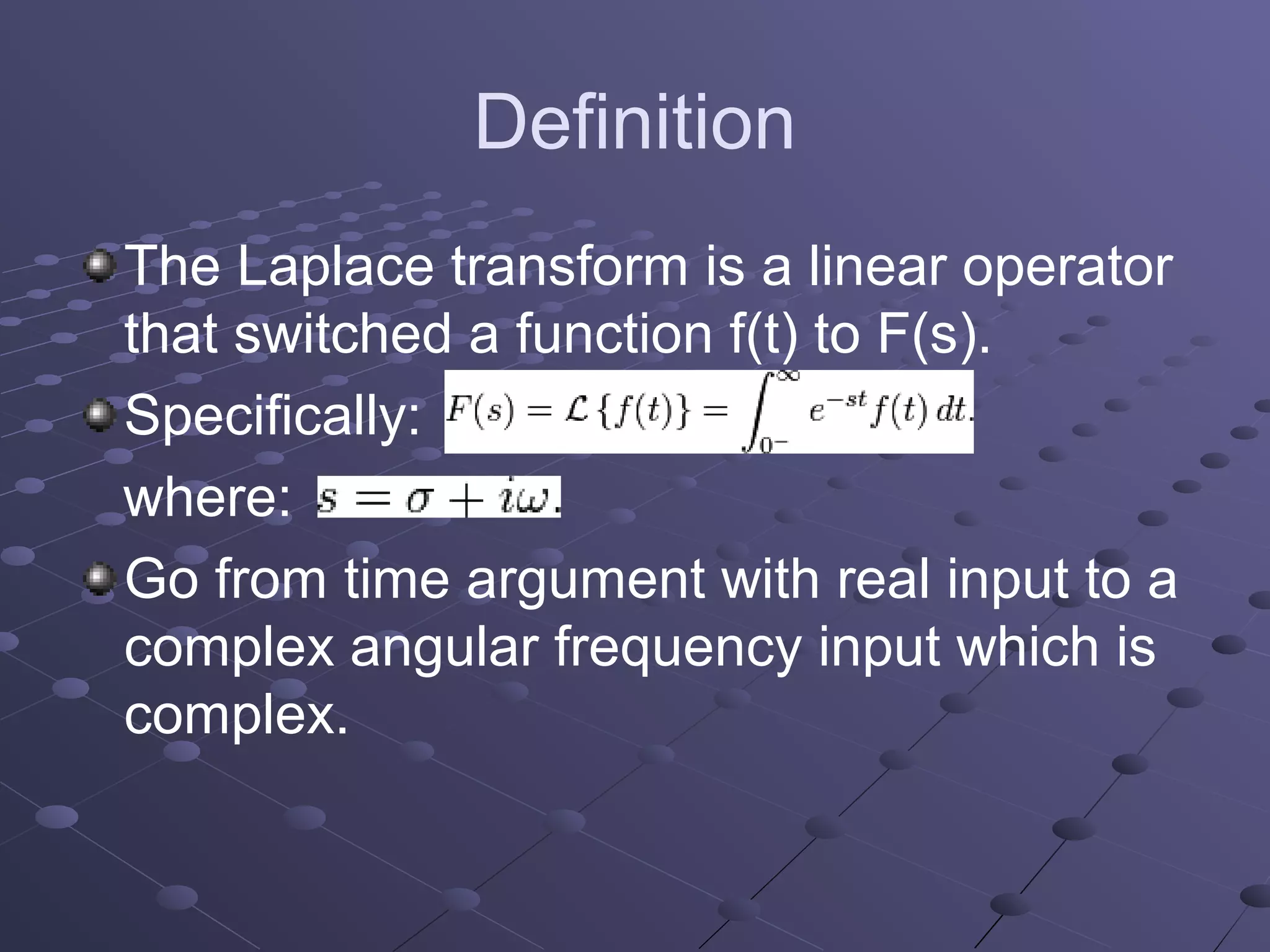
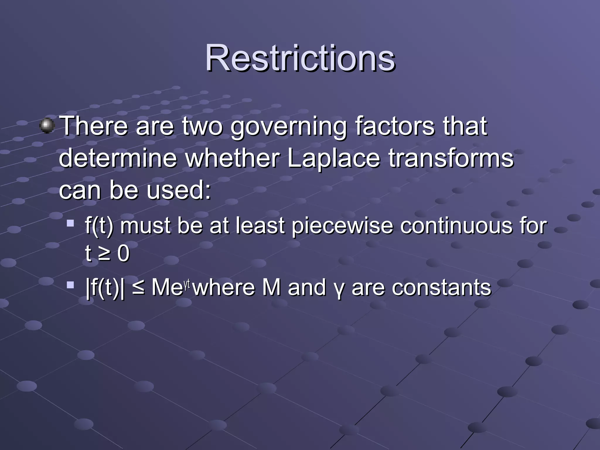
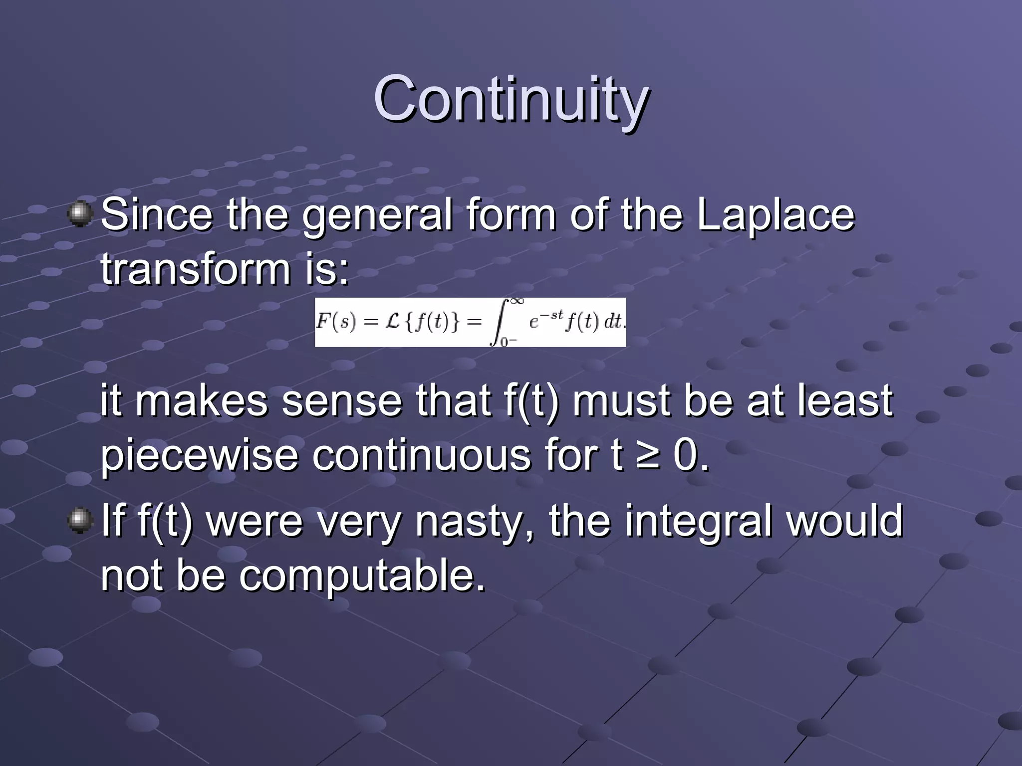
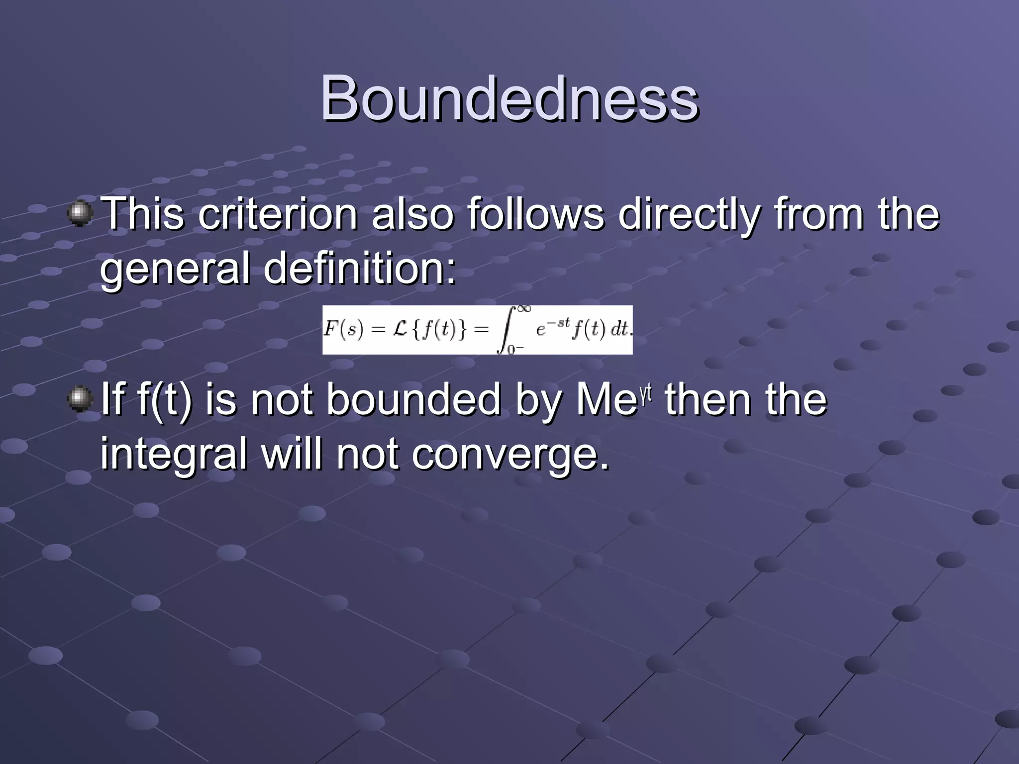
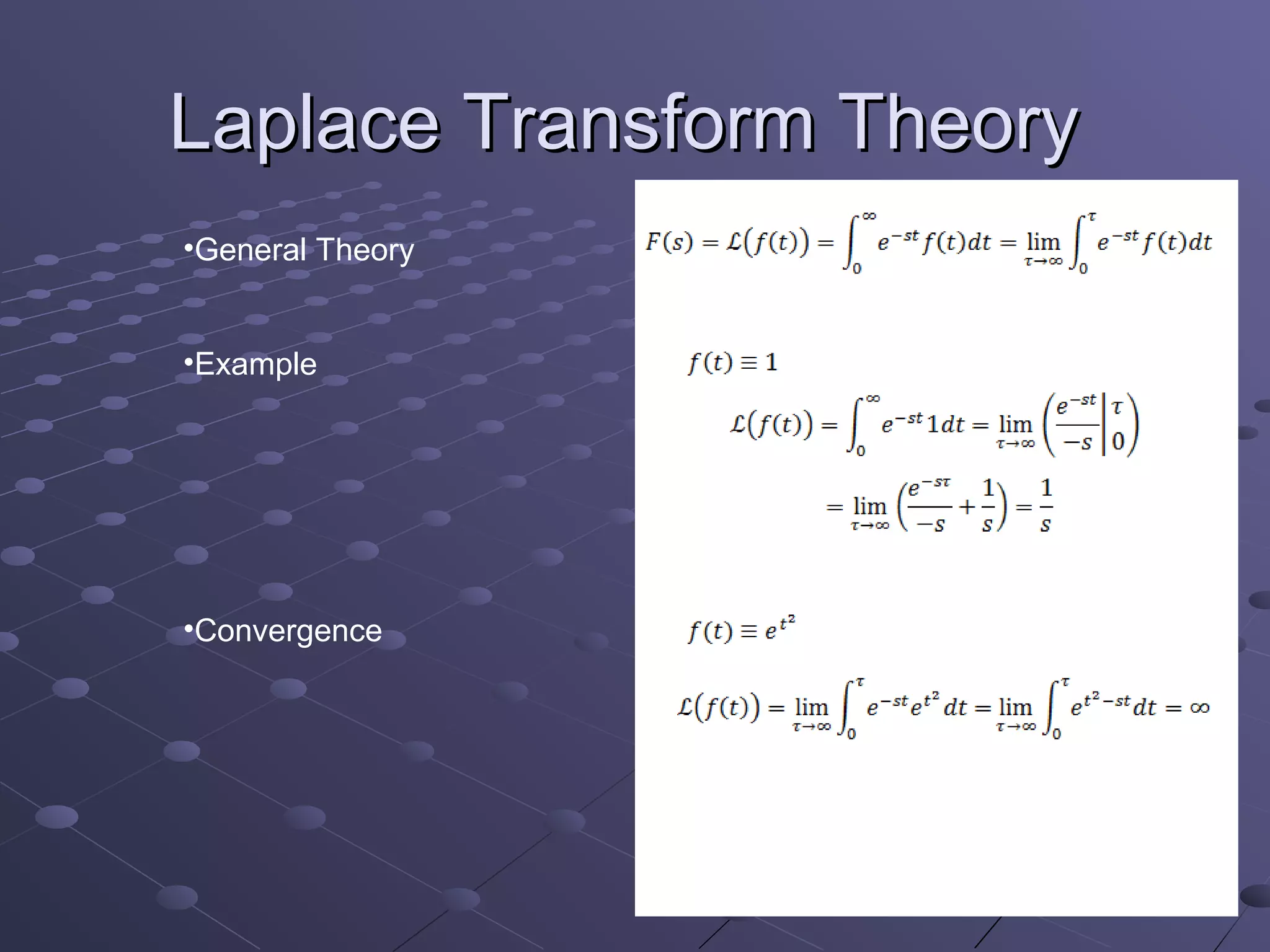
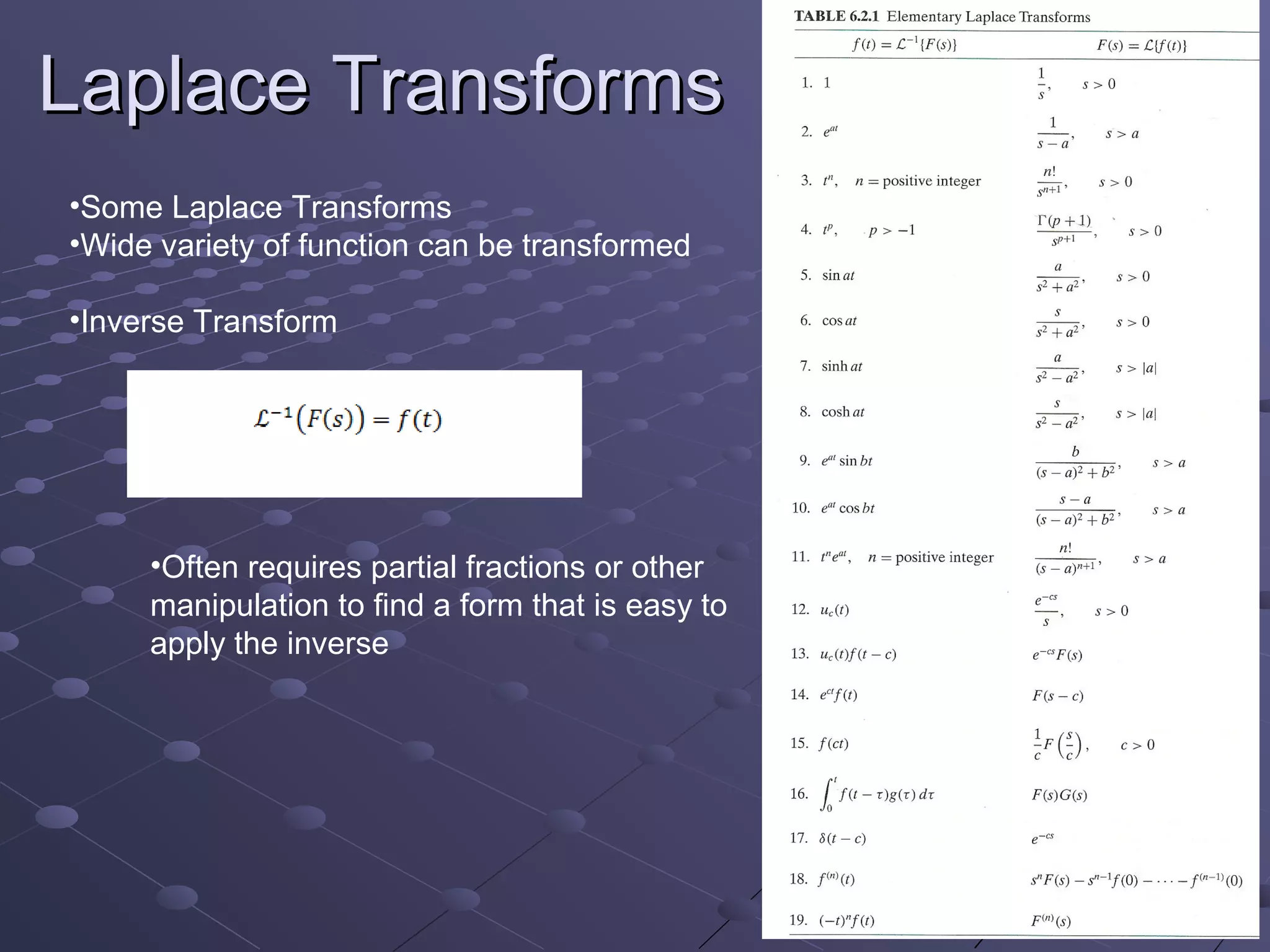
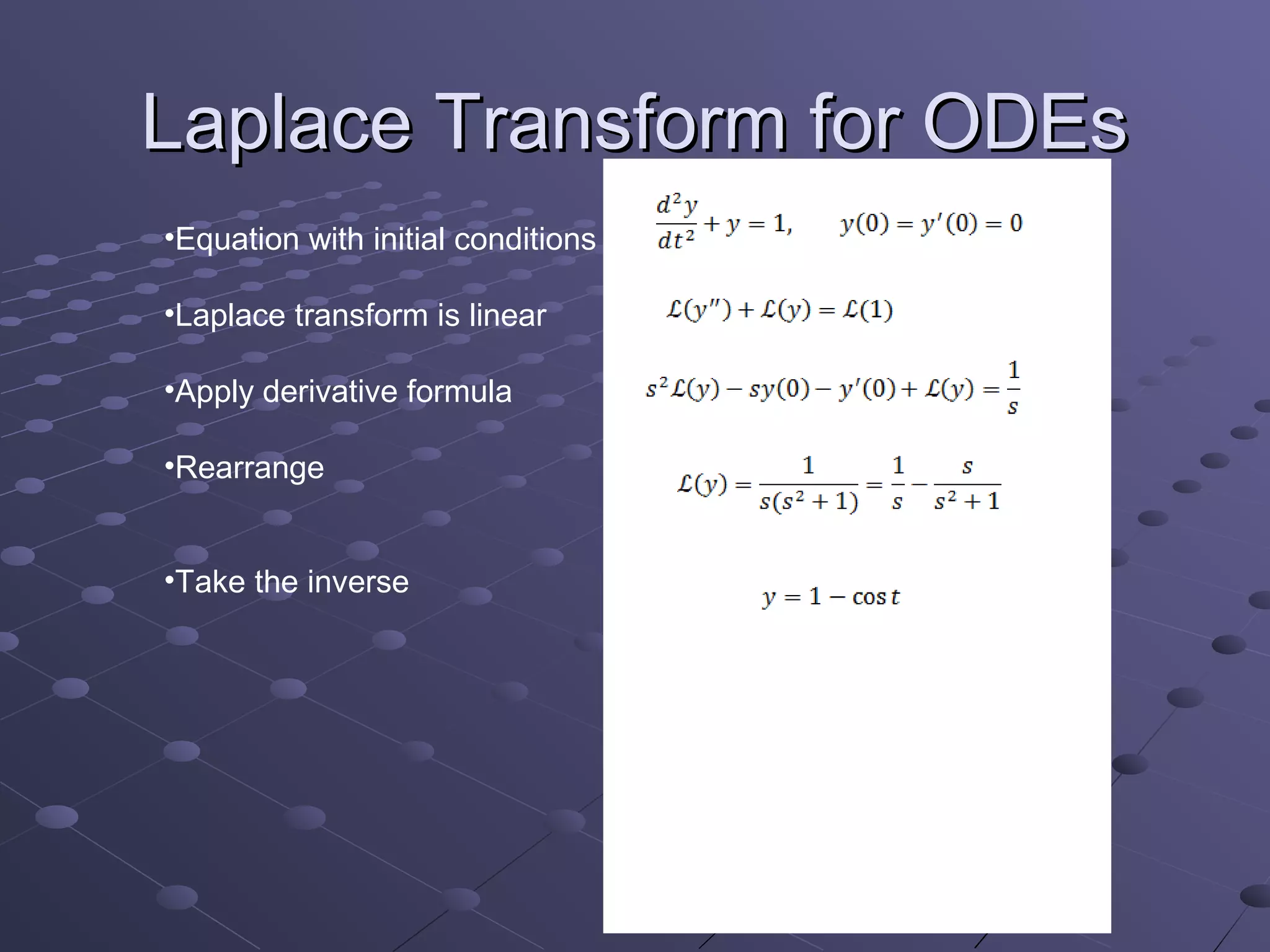
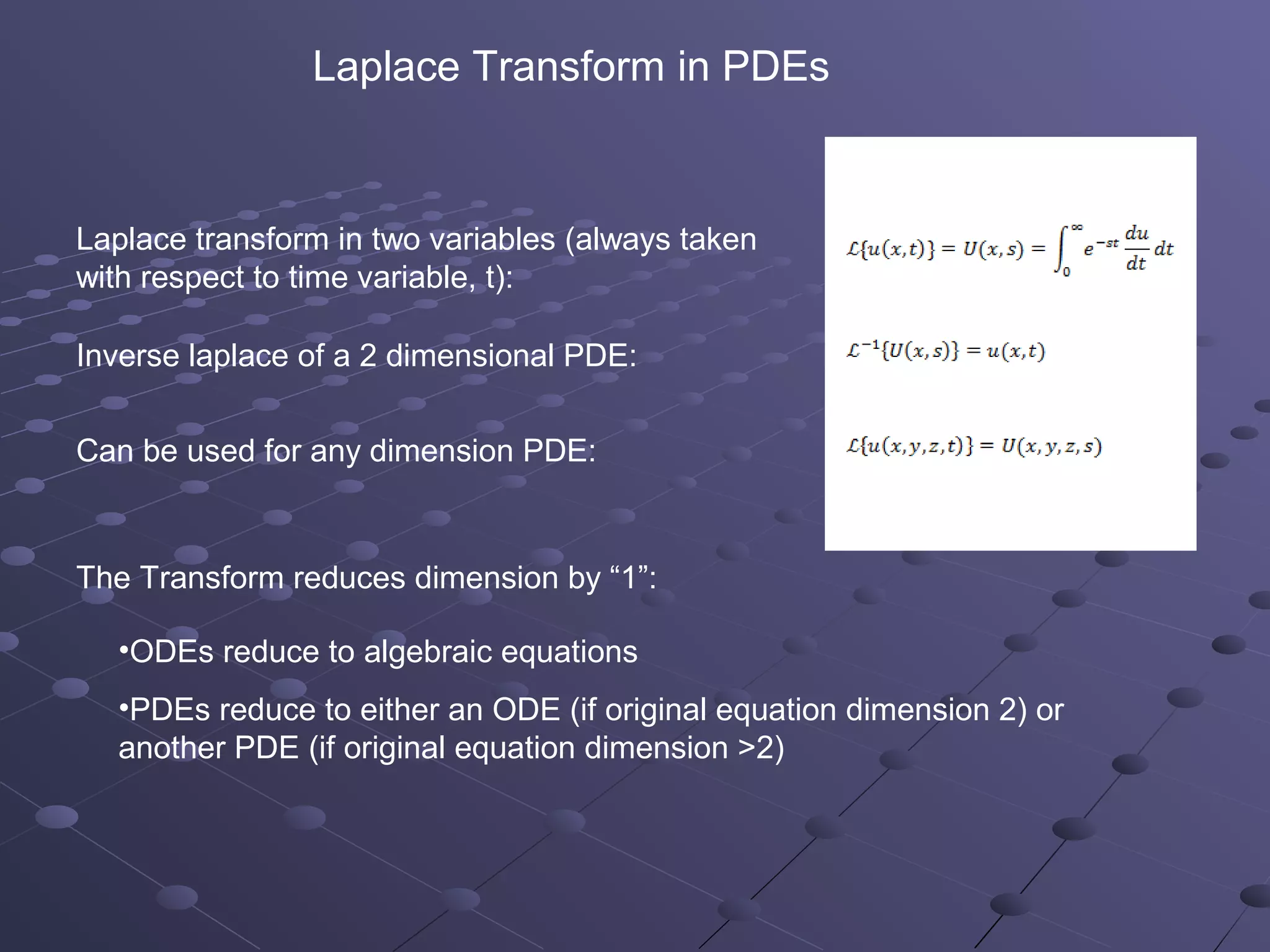
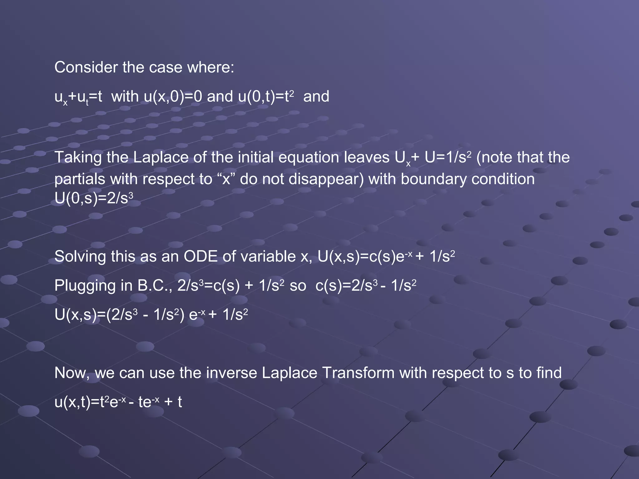
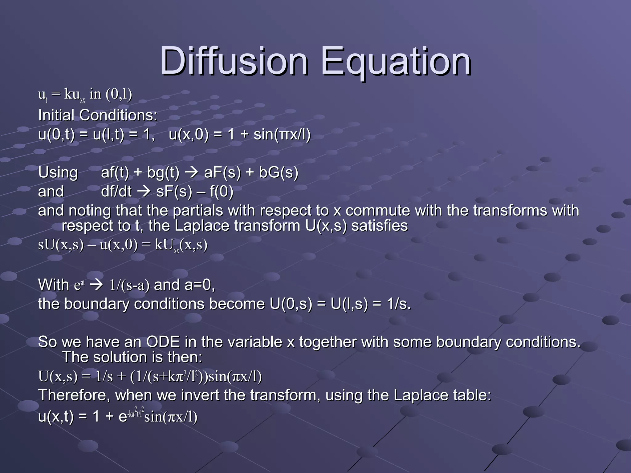
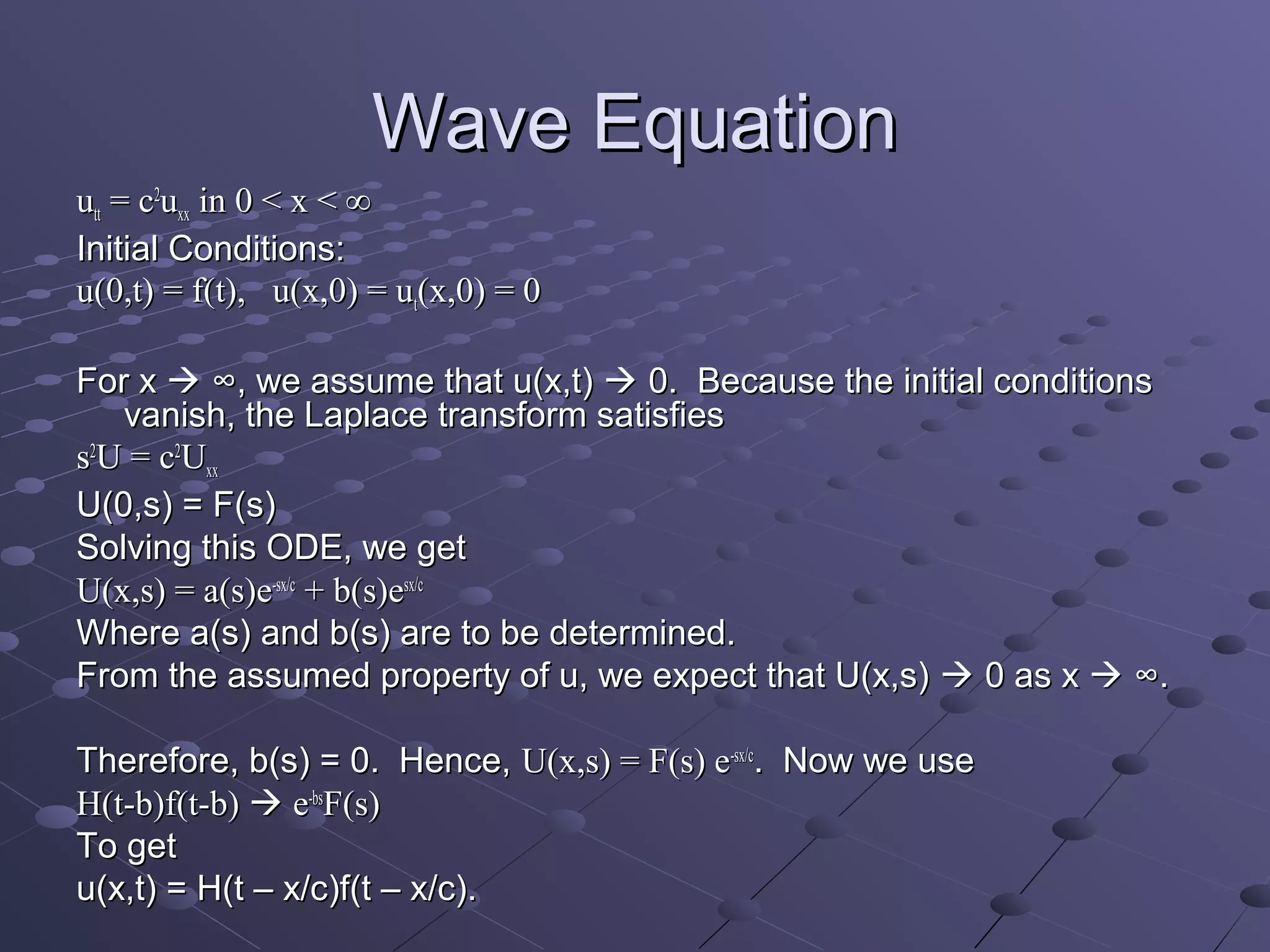
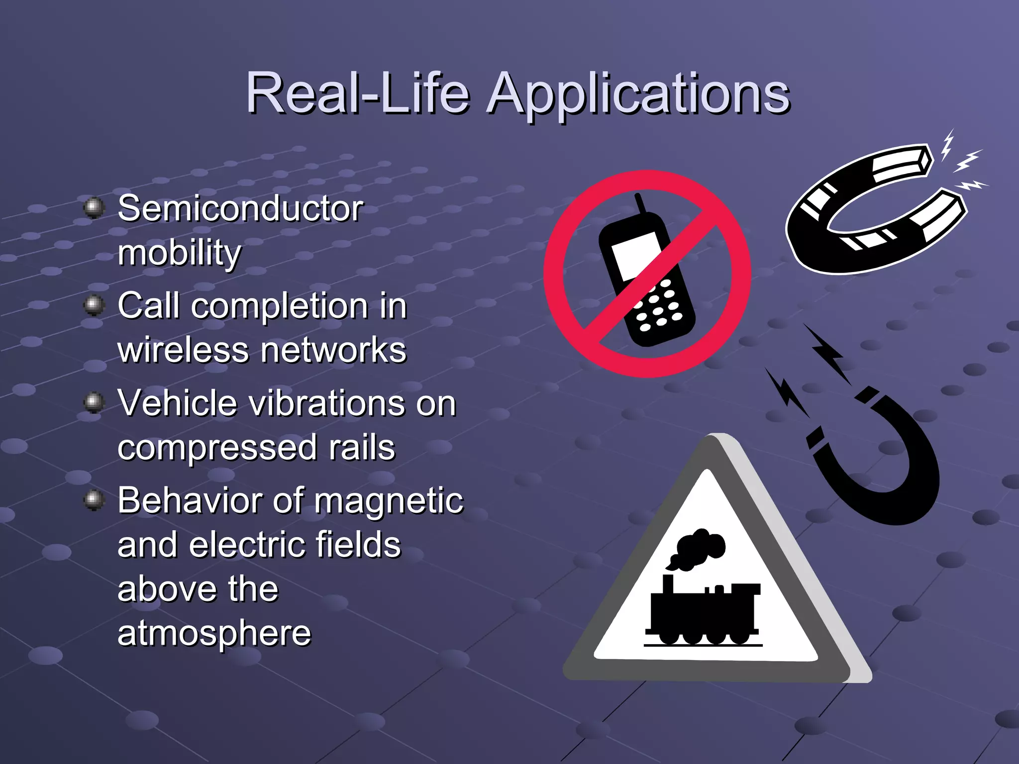
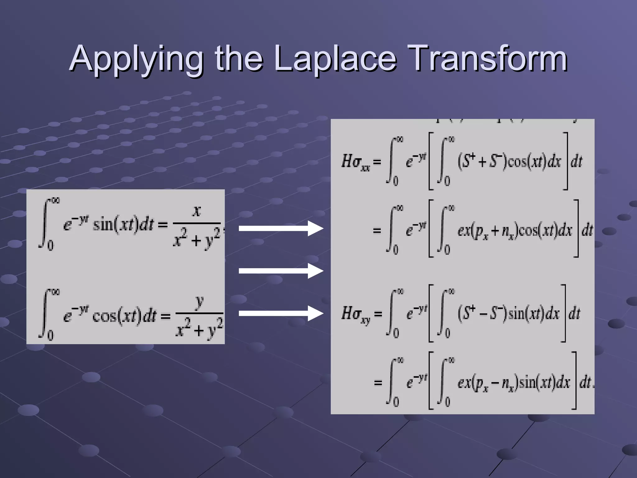
The document discusses the Laplace transform and its applications. Specifically: - The Laplace transform was developed by mathematicians including Euler, Lagrange, and Laplace to solve differential equations. - It transforms a function of time to a function of complex frequencies, allowing differential equations to be written as algebraic equations. - For a function to have a Laplace transform, it must be at least piecewise continuous and bounded above by an exponential function. - The Laplace transform can reduce the dimension of partial differential equations and is used in applications including semiconductor mobility, wireless networks, vehicle vibrations, and electromagnetic fields.

1. Laplace Transform
Naveen Sihag

2. The French Newton
Pierre-Simon Laplace
Developed mathematics in
astronomy, physics, and statistics
Began work in calculus which led
to the Laplace Transform
Focused later on celestial
mechanics
One of the first scientists to
suggest the existence of black
holes

3. History of the Transform
Euler began looking at integrals as solutions to differential equations
in the mid 1700’s:
Lagrange took this a step further while working on probability
density functions and looked at forms of the following equation:
Finally, in 1785, Laplace began using a transformation to solve
equations of finite differences which eventually lead to the current
transform

4. Definition
The Laplace transform is a linear operator
that switched a function f(t) to F(s).
Specifically:
where:
Go from time argument with real input to a
complex angular frequency input which is
complex.

5. Restrictions
There are two governing factors that
determine whether Laplace transforms
can be used:
 f(t) must be at least piecewise continuous for
t≥0

|f(t)| ≤ Meγt where M and γ are constants

6. Continuity
Since the general form of the Laplace
transform is:
it makes sense that f(t) must be at least
piecewise continuous for t ≥ 0.
If f(t) were very nasty, the integral would
not be computable.

7. Boundedness
This criterion also follows directly from the
general definition:
If f(t) is not bounded by Meγt then the
integral will not converge.

8. Laplace Transform Theory
•General Theory
•Example
•Convergence

9. Laplace Transforms
•Some Laplace Transforms
•Wide variety of function can be transformed
•Inverse Transform
•Often requires partial fractions or other
manipulation to find a form that is easy to
apply the inverse

10. Laplace Transform for ODEs
•Equation with initial conditions
•Laplace transform is linear
•Apply derivative formula
•Rearrange
•Take the inverse

11. Laplace Transform in PDEs
Laplace transform in two variables (always taken
with respect to time variable, t):
Inverse laplace of a 2 dimensional PDE:
Can be used for any dimension PDE:
The Transform reduces dimension by “1”:
•ODEs reduce to algebraic equations
•PDEs reduce to either an ODE (if original equation dimension 2) or
another PDE (if original equation dimension >2)

12. Consider the case where:
ux+ut=t with u(x,0)=0 and u(0,t)=t2 and
Taking the Laplace of the initial equation leaves Ux+ U=1/s2 (note that the
partials with respect to “x” do not disappear) with boundary condition
U(0,s)=2/s3
Solving this as an ODE of variable x, U(x,s)=c(s)e-x + 1/s2
Plugging in B.C., 2/s3=c(s) + 1/s2 so c(s)=2/s3 - 1/s2
U(x,s)=(2/s3 - 1/s2) e-x + 1/s2
Now, we can use the inverse Laplace Transform with respect to s to find
u(x,t)=t2e-x - te-x + t

13. Example Solutions

14. Diffusion Equation
ut = kuxx in (0,l)
Initial Conditions:
u(0,t) = u(l,t) = 1, u(x,0) = 1 + sin(πx/l)
Using af(t) + bg(t)  aF(s) + bG(s)
and df/dt  sF(s) – f(0)
and noting that the partials with respect to x commute with the transforms with
respect to t, the Laplace transform U(x,s) satisfies
sU(x,s) – u(x,0) = kUxx(x,s)
With eat  1/(s-a) and a=0,
the boundary conditions become U(0,s) = U(l,s) = 1/s.
So we have an ODE in the variable x together with some boundary conditions.
The solution is then:
U(x,s) = 1/s + (1/(s+kπ2/l2))sin(πx/l)
Therefore, when we invert the transform, using the Laplace table:
2 2
u(x,t) = 1 + e-kπ t/l sin(πx/l)

15. Wave Equation
utt = c2uxx in 0 < x < ∞
Initial Conditions:
u(0,t) = f(t), u(x,0) = ut(x,0) = 0
For x  ∞, we assume that u(x,t)  0. Because the initial conditions
vanish, the Laplace transform satisfies
s2U = c2Uxx
U(0,s) = F(s)
Solving this ODE, we get
U(x,s) = a(s)e-sx/c + b(s)esx/c
Where a(s) and b(s) are to be determined.
From the assumed property of u, we expect that U(x,s)  0 as x  ∞.
Therefore, b(s) = 0. Hence, U(x,s) = F(s) e-sx/c. Now we use
H(t-b)f(t-b)  e-bsF(s)
To get
u(x,t) = H(t – x/c)f(t – x/c).

16. Real-Life Applications
Semiconductor
mobility
Call completion in
wireless networks
Vehicle vibrations on
compressed rails
Behavior of magnetic
and electric fields
above the
atmosphere

17. Ex. Semiconductor Mobility
Motivation
 semiconductors are commonly
made with superlattices having
layers of differing compositions
 need to determine properties of
carriers in each layer
concentration of electrons and
holes
mobility of electrons and holes
 conductivity tensor can be related
to Laplace transform of electron
and hole densities

18. Notation
R = ratio of induced electric field to the product of
the current density and the applied magnetic field
ρ = electrical resistance
H = magnetic field
J = current density
E = applied electric field
n = concentration of electrons
u = mobility

19. Equation Manipulation
and

20. Assuming a continuous mobility
distribution and that ,
, it follows:

21. Applying the Laplace Transform

22. Source
Johnson, William B. Transform method for
semiconductor mobility, Journal of Applied
Physics 99 (2006).