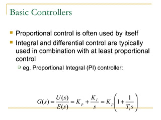
Downloaded 1,280 times


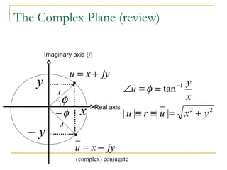
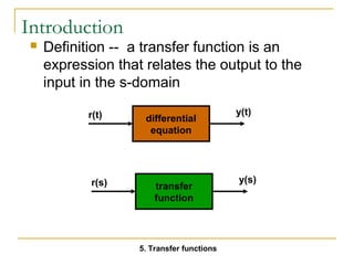
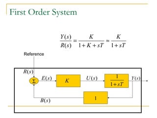
![Basic Tool For Continuous Time:
Laplace Transform
= = ò¥ -
L[ f (t)] F(s) f (t)e stdt
0
Convert time-domain functions and operations into
frequency-domain
f(t) ® F(s) (tÎR, sÎC)
Linear differential equations (LDE) ® algebraic expression
in Complex plane
Graphical solution for key LDE characteristics
Discrete systems use the analogous z-transform](https://image.slidesharecdn.com/laplacetransforms1-140923050517-phpapp01/85/Laplace-transforms-5-320.jpg)

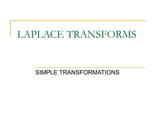
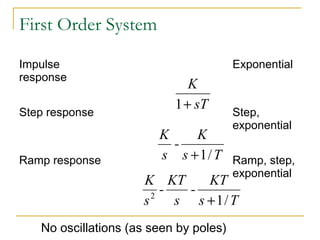
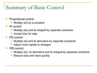
![Laplace Transform Properties
L af t bf t aF s bF s
[ ( ) ( )] ( ) ( )
L d
f t sF s f
dt
± - = úû
( ) ( ) (0 )
é
[ ] [ ]
L f t dt F s
( ) ( ) 1 ( )
f t dt
ò = +
ò
s s
f (t - τ)f (τ dτ =
F s F s
) ( ) ( )
Addition/Scaling
Differentiation
Integratio n
Convolution
Initial value theorem
- f + =
sF s
(0 ) lim ( )
s
®¥
lim ( ) lim ( )
0
0
1 2 1 2
0
1 2 1 2
- f t sF s
t s
t
t
®¥ ®
= ±
=
ù
êë
± = ±
ò
Final value theorem](https://image.slidesharecdn.com/laplacetransforms1-140923050517-phpapp01/85/Laplace-transforms-8-320.jpg)


![Different terms of 1st degree
To separate a fraction into partial fractions
when its denominator can be divided into
different terms of first degree, assume an
unknown numerator for each fraction
Example --
(11x-1)/(X2 - 1) = A/(x+1) + B/(x-1)
= [A(x-1) +B(x+1)]/[(x+1)(x-1))]
A+B=11
-A+B=-1
A=6, B=5](https://image.slidesharecdn.com/laplacetransforms1-140923050517-phpapp01/85/Laplace-transforms-19-320.jpg)

![Different quadratic terms
When there is a quadratic term, assume a
numerator of the form Ax + B
Example --
1/[(x+1) (x2 + x + 2)] = A/(x+1) + (Bx +C)/ (x2 +
x + 2)
1 = A (x2 + x + 2) + Bx(x+1) + C(x+1)
1 = (A+B) x2 + (A+B+C)x +(2A+C)
A+B=0
A+B+C=0
2A+C=1
A=0.5, B=-0.5, C=0
3. Partial fractions](https://image.slidesharecdn.com/laplacetransforms1-140923050517-phpapp01/85/Laplace-transforms-22-320.jpg)
![Repeated quadratic terms
Example --
1/[(x+1) (x2 + x + 2)2] = A/(x+1) + (Bx +C)/ (x2 +
x + 2) + (Dx +E)/ (x2 + x + 2)2
1 = A(x2 + x + 2)2 + Bx(x+1) (x2 + x + 2) +
C(x+1) (x2 + x + 2) + Dx(x+1) + E(x+1)
A+B=0
2A+2B+C=0
5A+3B+2C+D=0
4A+2B+3C+D+E=0
4A+2C+E=1
A=0.25, B=-0.25, C=0, D=-0.5, E=0
3. Partial fractions](https://image.slidesharecdn.com/laplacetransforms1-140923050517-phpapp01/85/Laplace-transforms-23-320.jpg)
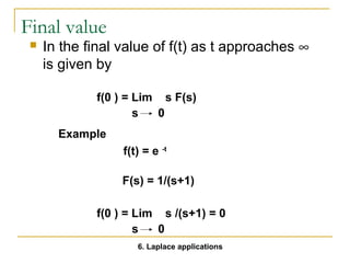
![Apply Initial- and Final-Value
Theorems to this Example
Laplace
transform of the
function.
Apply final-value
theorem
Apply initial-value
theorem
( ) 2
=
s s s
+ +
( 2) ( 4)
Y s
lim ( ) 2(0) =
[ ]
1
4
+ +
(0) (0 2) (0 4)
= ®¥ f t t
= ¥ ® f t t
lim ( ) 2( ) 0 =
[ ] 0
¥ ¥+ ¥+
( ) ( 2) ( 4)](https://image.slidesharecdn.com/laplacetransforms1-140923050517-phpapp01/85/Laplace-transforms-24-320.jpg)


![Solution process (4 of 8)
Step 3: Use table of transforms to express
equation in s-domain
L{D2 y} + L{2D y} + L{2y} = L{cos w t}
L{D2 y} = s2 Y(s) - sy(0) - D y(0)
L{2D y} = 2[ s Y(s) - y(0)]
L{2y} = 2 Y(s)
L{cos t} = s/(s2 + 1)
s2 Y(s) - s + 2s Y(s) - 2 + 2 Y(s) = s /(s2 + 1)](https://image.slidesharecdn.com/laplacetransforms1-140923050517-phpapp01/85/Laplace-transforms-29-320.jpg)
![Solution process (5 of 8)
Step 4: Solve for Y(s)
s2 Y(s) - s + 2s Y(s) - 2 + 2 Y(s) = s/(s2 + 1)
(s2 + 2s + 2) Y(s) = s/(s2 + 1) + s + 2
Y(s) = [s/(s2 + 1) + s + 2]/ (s2 + 2s + 2)
= (s3 + 2 s2 + 2s + 2)/[(s2 + 1) (s2 + 2s + 2)]](https://image.slidesharecdn.com/laplacetransforms1-140923050517-phpapp01/85/Laplace-transforms-30-320.jpg)
![Solution process (6 of 8)
Step 5: Expand equation into format covered by
table
Y(s) = (s3 + 2 s2 + 2s + 2)/[(s2 + 1) (s2 + 2s + 2)]
= (As + B)/ (s2 + 1) + (Cs + E)/ (s2 + 2s + 2)
(A+C)s3 + (2A + B + E) s2 + (2A + 2B + C)s + (2B
+E)
1 = A + C
2 = 2A + B + E
2 = 2A + 2B + C
2 = 2B + E
A = 0.2, B = 0.4, C = 0.8, E = 1.2](https://image.slidesharecdn.com/laplacetransforms1-140923050517-phpapp01/85/Laplace-transforms-31-320.jpg)
![Solution process (7 of 8)
(0.2s + 0.4)/ (s2 + 1)
= 0.2 s/ (s2 + 1) + 0.4 / (s2 + 1)
(0.8s + 1.2)/ (s2 + 2s + 2)
= 0.8 (s+1)/[(s+1)2 + 1] + 0.4/ [(s+1)2 + 1]](https://image.slidesharecdn.com/laplacetransforms1-140923050517-phpapp01/85/Laplace-transforms-32-320.jpg)
![Solution process (8 of 8)
Step 6: Use table to convert s-domain to
time domain
0.2 s/ (s2 + 1) becomes 0.2 cos t
0.4 / (s2 + 1) becomes 0.4 sin t
0.8 (s+1)/[(s+1)2 + 1] becomes 0.8 e-t cos t
0.4/ [(s+1)2 + 1] becomes 0.4 e-t sin t
y(t) = 0.2 cos t + 0.4 sin t + 0.8 e-t cos t + 0.4 e-t
sin t](https://image.slidesharecdn.com/laplacetransforms1-140923050517-phpapp01/85/Laplace-transforms-33-320.jpg)
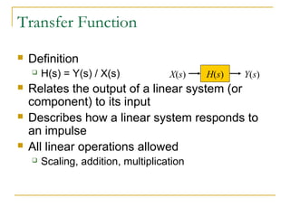


![Example
v(t)
R
C
L
v(t) = R I(t) + 1/C I(t) dt + L di(t)/dt
V(s) = [R I(s) + 1/(C s) I(s) + s L I(s)]
Note: Ignore initial conditions
5. Transfer functions](https://image.slidesharecdn.com/laplacetransforms1-140923050517-phpapp01/85/Laplace-transforms-39-320.jpg)


![Apply Initial- and Final-Value
Theorems to this Example
Laplace
transform of the
function.
Apply final-value
theorem
Apply initial-value
theorem
( ) 2
=
s s s
+ +
( 2) ( 4)
Y s
lim ( ) 2(0) =
[ ]
1
4
+ +
(0) (0 2) (0 4)
= ®¥ f t t
= ¥ ® f t t
lim ( ) 2( ) 0 =
[ ] 0
¥ ¥+ ¥+
( ) ( 2) ( 4)](https://image.slidesharecdn.com/laplacetransforms1-140923050517-phpapp01/85/Laplace-transforms-58-320.jpg)
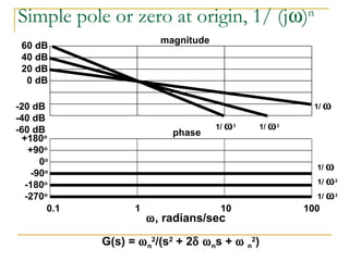
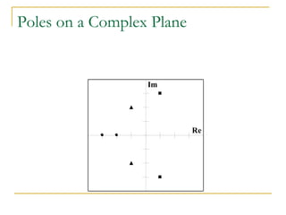
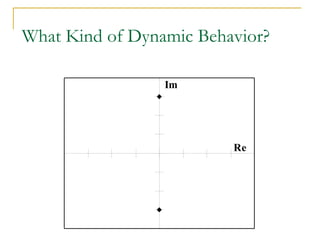
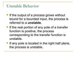
![Poles
The poles of a Laplace function are the
values of s that make the Laplace function
evaluate to infinity. They are therefore the
roots of the denominator polynomial
10 (s + 2)/[(s + 1)(s + 3)] has a pole at s =
-1 and a pole at s = -3
Complex poles always appear in complex-conjugate
pairs
The transient response of system is
determined by the location of poles
6. Laplace applications](https://image.slidesharecdn.com/laplacetransforms1-140923050517-phpapp01/85/Laplace-transforms-59-320.jpg)
![Zeros
The zeros of a Laplace function are the
values of s that make the Laplace function
evaluate to zero. They are therefore the
zeros of the numerator polynomial
10 (s + 2)/[(s + 1)(s + 3)] has a zero at s =
-2
Complex zeros always appear in complex-conjugate
pairs
6. Laplace applications](https://image.slidesharecdn.com/laplacetransforms1-140923050517-phpapp01/85/Laplace-transforms-60-320.jpg)


![Derivation of a Transfer Function
T s = F T s +
F T s
1 1 2 2 ( ) ( ) ( )
F
1
[ 1 2 ]
G s T s
( ) ( )
1 ( )
M s F F
T s
+ +
= =
Apply Laplace transform
to each term considering
that only inlet and outlet
temperatures change.
Determine the transfer
function for the effect of
inlet temperature
changes on the outlet
temperature.
Note that the response
is first order.
[ M s + F +
F
] 1 2](https://image.slidesharecdn.com/laplacetransforms1-140923050517-phpapp01/85/Laplace-transforms-74-320.jpg)


This document provides an overview of Laplace transforms. Key points include: - Laplace transforms convert differential equations from the time domain to the algebraic s-domain, making them easier to solve. The process involves taking the Laplace transform of each term in the differential equation. - Common Laplace transforms of functions are presented. Properties such as linearity, differentiation, integration, and convolution are also covered. - Partial fraction expansion is used to break complex fractions in the s-domain into simpler forms with individual terms that can be inverted using tables of transforms. - Solving differential equations using Laplace transforms follows a standard process of taking the Laplace transform of each term, rewriting the equation in the s-domain, solving