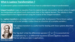
The Laplace transform is an integral transform that converts a function of time (often a function that represents a signal) into a function of complex frequency. It has various applications in engineering for solving differential equations and analyzing linear systems. The key aspect is that it converts differential operators into algebraic operations, allowing differential equations to be solved as algebraic equations. This makes the equations much easier to manipulate and solve compared to the original differential form.

2. To understand Laplace transformation first we have to understand integral transformation.
Integral transform maps an equation from its original domain into another domain where it might
be manipulated and solved much more easily than in the original domain. The solution is then
mapped back to the original domain using the inverse of the integral transform.
So, Laplace transform is an integral transform named after its discoverer Pierre-Simon Laplace
It takes a function of a real variable t (often time) to a function of a complex variable s.
The Laplace transform is a useful tool for dealing with linear systems described
by ODEs.
The 'big deal' is that the differential operator ('
𝑑
𝑑𝑥
' or '
𝑑
𝑑𝑡
') is converted into
multiplication by 's', so differential equations become algebraic equations.
That we will discuss later in applications.
Pierre-Simon Laplace

3. If 𝑓 𝑡 is a function of t for all t≥0 then 0
∞
𝑒−𝑠𝑡 𝑓 𝑡 𝑑𝑡 is defined as the laplace transform of
𝑓 𝑡 ,provided integral exists and denoted by L{𝑓 𝑡 }.
(1) 𝑓 𝑡 is piecewise continuous function.
(2) lim
𝑡→∞
{𝑒−𝛼𝑡 𝑓 𝑡 }= Finite quantity. ( t≥0 ).
By using 0
∞
𝑒−𝑠𝑡 𝑓 𝑡 𝑑𝑡 we can find laplace transform of any function. Here are some standard
Laplace transforms which can further be used to evaluate Laplace transform of other complex
Functions.
Note that, To evaluate Laplace transform some special functions like Gamma function, Beta
Function etc. are also used.

4. Laplace transform of some basic functions

5. If L{𝑓 𝑡 }=F(s) and L{𝑔 𝑡 }=G(s) then, L{a𝑓 𝑡 + b𝑔 𝑡 }= a F(s)+b G(s).
Where a and b are constants.
If L{𝑓 𝑡 }=F(s) then L{𝑓 𝑎𝑡 }=
1
𝑎
F
𝑠
𝑎
.
If L{𝑓 𝑡 } = F(s) then L{𝑒−𝑎𝑡
𝑓 𝑡 } = F(s + a).
If L{𝑓 𝑡 } = F(s)
And g 𝑡 =
𝑓 𝑡 − 𝑎 , 𝑡 > 𝑎
0 , 𝑡 < 𝑎
then L{g 𝑡 }=𝑒−𝑎𝑠 𝐹 𝑠 .

6. If L{𝑓 𝑡 } = F(s) then L{𝑡 𝑛
𝑓 𝑡 } = (−1) 𝑛 𝑑 𝑛
𝑑𝑠 𝑛F(s).
If L{𝑓 𝑡 } = F(s) then L
𝑓(𝑡)
𝑡 𝑛 = 𝑠
∞
𝑠
∞
… 𝑛 𝑡𝑖𝑚𝑒𝑠 𝐹 𝑠 𝑑𝑠.
If L{𝑓 𝑡 } = F(s) then L{ 0
𝑡
𝑓(𝑡)} =
𝐹(𝑆)
𝑠
.
Unit step function is defined as, u 𝑡 =
0, 𝑡 < 0
1, 𝑡 > 0
,unit step function is also known as
heaviside function.
Now, delayed unit step function can be defined as, u 𝑡 − 𝑡0 =
0, 𝑡 < 𝑡0
1, 𝑡 > 𝑡0
L{𝑓 𝑡 𝑢(𝑡 − 𝑡0)} = 𝑒−𝑡0 𝑠 𝐹 𝑠 + 𝑡0 , where L{𝑓 𝑡 } = F(s) .

7. Graph of unit step function Graph of delayed unit step function
A function 𝑓(𝑡) is said to be periodic if there exists a constant (T>0) such that 𝑓 𝑡 + 𝑡 = 𝑓(𝑡)
For all values of t.
In general, 𝑓 𝑡 + 𝑛𝑇 = 𝑓(𝑡) for all t, where n is an integer (positive or negative).
If 𝑓 𝑡 is a piecewise continuous function with period T then L{𝑓 𝑡 } =
1
1−𝑒−𝑇𝑠 0
𝑇
𝑒−𝑠𝑡 𝑓 𝑡 𝑑𝑡.

8. Consider the following function: 𝑓 𝑡 =
−
1
𝑇
,
−𝑇
2
< 𝑡 <
𝑇
2
0, 𝑜𝑡ℎ𝑒𝑟𝑤𝑖𝑠𝑒
The width of this function is T and its amplitude is 1/T. Hence, the are of this function is 1 unit.
As 𝑇 → 0, this function becomes a delta function or a unit impulse function.
Dirac’s delta function has zero amplitude everywhere except at t=0. At t=0 amplitude of the
function is infinitely large such that are under its curve equals to 1 unit. Hence delta function
can be defined as,
𝛿 𝑡 = 0, 𝑡 ≠ 0
−∞
∞
𝛿 𝑡 𝑑𝑡 = 1 𝑡 = 0
And,
The displaced (delayed) delta or unit impulse function 𝛿(𝑡 − 𝑎) represents the function 𝛿 𝑡
which is displaced by a distance ‘a’ to the right.
lim
𝑇→0
𝑓 𝑡 = 𝛿(𝑡)

9. Delayed delta function: 𝛿 𝑡 − 𝑎 = 0, 𝑡 ≠ 0
−∞
∞
𝛿 𝑡 − 𝑎 𝑑𝑡 = 1 𝑡 = 0
Now, L 𝑓 𝑡 𝛿 𝑡 − 𝑎 = 𝑒−𝑎𝑠 𝑓 𝑎 .
Graph of delta function Animated explanation of
delta function

10. If L{𝑓 𝑡 } = F(s) then 𝑓 𝑡 is called the inverse Laplace transform of F(s). Mathematically it is
Written as : 𝑓 𝑡 =𝐿−1
𝐹(𝑠) . Where 𝐿−1
is called inverse Laplace operator.
Note that, 𝑓 𝑡 is the piecewise-continuous and exponentially-restricted real function.
Inverse Laplace transforms of simple functions can be found from the properties of Laplace
transforms.

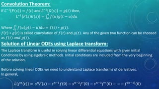
11. If 𝐿−1
{F 𝑠 } = 𝑓(𝑡) then 𝐿−1
{F(s + a)} = 𝑒−𝑎𝑡
𝑓 𝑡 .
If 𝐿−1
{F 𝑠 } = 𝑓(𝑡)
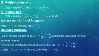
And g 𝑡 =
𝑓 𝑡 − 𝑎 , 𝑡 > 𝑎
0 , 𝑡 < 𝑎
then 𝐿−1 {𝑒−𝑎𝑠 𝐹 𝑠 } = 𝑔 𝑡 .
If 𝐿−1 {F 𝑠 } = 𝑓 𝑡 then 𝐿−1 {sF 𝑠 } = 𝑓′(𝑡) =
𝑑
𝑑𝑡
[𝐿−1 {F 𝑠 }].
In general, 𝐿−1 {𝑠 𝑛F 𝑠 } = 𝑓 𝑛(𝑡).
If 𝐿−1
{F 𝑠 } = 𝑓 𝑡 then 𝐿−1
{
𝐹(𝑠)
𝑠
} = 0
𝑡
𝑓 𝑡 𝑑𝑡.
In general, 𝐿−1 {
𝐹(𝑠)
𝑠 𝑛 } = 0
𝑡
0
𝑡
0
𝑡
… 𝑛 𝑡𝑖𝑚𝑒𝑠 𝑓 𝑡 𝑑𝑡 𝑑𝑡 𝑑𝑡 … 𝑛 𝑡𝑖𝑚𝑒𝑠.

12. If 𝐿−1
{F 𝑠 } = 𝑓(𝑡) then 𝐿−1
{𝐹(𝑠)} =
−1
𝑡
𝐿−1
{𝐹′
(𝑠)}.
Sometimes it is hard to find inverse Laplace transforms directly. We can use this method to find
Inverse Laplace transform easily. For ex: log , Trignomatric inverse functions .
If 𝐿−1{F 𝑠 } = 𝑓(𝑡) then 𝐿−1{𝐹(𝑠)} = 𝐿−1{ 𝑠
∞
𝐹 𝑠 𝑑𝑠}.
This can be used for higher power terms in denominator. For ex:
2
(𝑠−𝑎)3 .
Sometimes given function has complex polynomials in denominator in That types of cases it is
hard to find Laplace transforms of them. For ex:
𝑠
(𝑠+1)(𝑠−1)(𝑠2+4)
.
Any function F(s) can be written as
𝑃(𝑠)
𝑄(𝑠)
, where P(s) and Q(s) are polynomials in s.
To perform partial fraction expansion, the degree of P(s) must be less than the degree of Q(s).
Assuming the degree of P(s) is less than that of Q(s), four possible cases arise depanding upon
The factors of Q(s).

13. Case 1 Factors are linear and distinct:
𝐹(𝑠) =
𝑃(𝑠)
(𝑠 + 𝑎)(𝑠 + 𝑏)
By partial fraction expansion,
𝐹(𝑠) =
𝐴
(𝑠 + 𝑎)
+
𝐵
(𝑠 + 𝑏)
Case 2 Factors are linear and repeated:
𝐹(𝑠) =
𝑃(𝑠)
(𝑠 + 𝑎)(𝑠 + 𝑏) 𝑛
𝐹 𝑠 =
𝐴
𝑠 + 𝑎
+
𝐵1
𝑠 + 𝑏
+
𝐵2
(𝑠 + 𝑏)2
+ ⋯ +
𝐵𝑛
(𝑠 + 𝑏) 𝑛
By partial fraction expansion

14. Case 3 Factors are quadratic and distinct:
𝐹(𝑠) =
𝑃(𝑠)
(𝑠2 + 𝑎𝑠 + 𝑏)(𝑠2 + 𝑐𝑠 + 𝑑)
By partial fraction expansion,
𝐹(𝑠) =
𝐴𝑠 + 𝐵
(𝑠2 + 𝑎𝑠 + 𝑏)
+
𝐶𝑠 + 𝐷
(𝑠2 + 𝑐𝑠 + 𝑑)
Case 4 Factors are quadratic and repeated:
𝐹(𝑠) =
𝑃(𝑠)
(𝑠2 + 𝑎𝑠 + 𝑏)(𝑠2 + 𝑐𝑠 + 𝑑) 𝑛
By partial fraction expansion,
𝐹 𝑠 =
𝐴𝑠 + 𝐵
𝑠2 + 𝑎𝑠 + 𝑏
+
𝐶1 𝑠 + 𝐷1
𝑠2 + 𝑐𝑠 + 𝑑
+
𝐶2 𝑠 + 𝐷2
(𝑠2 + 𝑐𝑠 + 𝑑)2
+ ⋯ +
𝐶 𝑛 𝑠 + 𝐷 𝑛
(𝑠2 + 𝑐𝑠 + 𝑑) 𝑛
.
Type equation here.
The constant coefficients can be found out by equating two sides equal and evaluating it. Thus
We can do partial expansion of given function and find inverse Laplace transform by linearity
Property.

15. If 𝐿−1 𝐹 𝑠 = 𝑓 𝑡 and 𝐿−1 𝐺 𝑠 = 𝑔 𝑡 then,
𝐿−1 𝐹 𝑠 𝐺(𝑠) = 0
𝑡
𝑓 𝑢 𝑔 𝑡 − 𝑢 𝑑𝑢
Where 0
𝑡
𝑓 𝑢 𝑔 𝑡 − 𝑢 𝑑𝑢 = 𝑓 𝑡 ∗ 𝑔(𝑡).
𝑓 𝑡 ∗ 𝑔 𝑡 is called convolution of 𝑓 𝑡 and 𝑔(𝑡). Any of the given two function can be choosed
as 𝑓 𝑡 𝑎𝑛𝑑 𝑔(𝑡).
The Laplace transform is useful in solving linear differential equations with given initial
Conditions by using algebraic methods. Initial conditions are included from the very beginning
of the solution.
Before solving linear ODEs we need to understand Laplace transforms of derivatives.
In general,
𝐿 𝑓 𝑛 𝑡 = 𝑠 𝑛 𝐹 𝑠 − 𝑠 𝑛−1 𝑓 0 − 𝑠 𝑛−2 𝑓′ 0 − 𝑠 𝑛−3 𝑓′′ 0 − ⋯ − 𝑓(𝑛−1) 0

16. From this formula we can derive expressions for any derivative of 𝑓(𝑡).
Linear
Differential
equation
Algebraic
equation
Solution of
Differential
equation
Solution of
algebraic
equation
Method for solving ODE
Laplace transform
Inverse
Laplace transform
By following method in the above figure we can solve any ODE easily. The drawback of this
method is that 𝑓 0 , 𝑓′ 0 , 𝑓′′ 0 𝑒𝑡𝑐. are required.

17. Basically, a Laplace transform will convert a function in some domain into a function in another
domain, without changing the value of the function. We use Laplace transform to convert
equations having complex differential equations to relatively simple equations having
polynomials. Since equations having polynomials are easier to solve, we employ Laplace
transform to make calculations easier.
We use Laplace transform on a derivative to convert it into a multiple of the domain variable.
Thus with Laplace transform 𝑛 𝑡ℎ degree differential equation can be transformed into an 𝑛 𝑡ℎ
degree polynomial. One can easily solve the polynomial to get the result and then change it into
a differential equation using inverse Laplace transform.
Laplace Transform is heavily used in signal processing. Using Laplace or Fourier transform, you
can study a signal in the frequency domain. This can be a powerful tool. For instance, if your
signal is smooth over time, it means that, in the frequency domain, you're very likely to find only
small frequencies.

18. Machine learning focuses on prediction, based on known properties learned from the training
data. Data mining (which is the analysis step of Knowledge Discovery in Databases) focuses on
the discovery of (previously) unknown properties on the data. Where Laplace equation is used
to determine the prediction and to analyses the step of knowledge in databases.
Laplace transform has several applications in almost all Engineering disciplines.
1) System Modelling
Laplace transform is used to simplify calculations in system modelling, where large differential
equations are used.
2) Analysis of Electrical Circuits
In electrical circuits, a Laplace transform is used for the analysis of linear time-invariant systems.
3) Analysis of Electronic Circuits
Laplace transform is widely used by Electronics engineers to quickly solve differential equations
occurring in the analysis of electronic circuits.
4) Digital Signal Processing
One cannot imagine solving DSP (Digital Signal processing) problems without employing Laplace
transform.

19. 5) Nuclear Physics
In order to get the true form of radioactive decay, a Laplace transform is used. It makes studying
analytic part of Nuclear Physics possible.
6) Process Controls
Laplace transforms are critical for process controls. It helps analyze the variables, which when
altered, produces desired manipulations in the result. For example, while study heat
experiments, Laplace transform is used to find out to what extent the given input can be altered
by changing temperature, hence one can alter temperature to get desired output for a while.
This is an efficient and easier way to control processes that are guided by differential equations.

20. https://en.wikipedia.org/wiki/Laplace_transform
https://en.wikipedia.org/wiki/Fourier_transform
https://en.wikipedia.org/wiki/Integral_transform
https://math.stackexchange.com/questions/181160/what-exactly-is-laplace-transform
https://en.wikipedia.org/wiki/Inverse_Laplace_transform
https://en.wikipedia.org/wiki/Dirac_delta_function
https://www.quora.com/What-are-the-real-world-applications-of-Laplace-transform-especially-in-computer-science