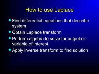
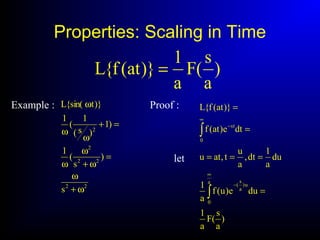
Laplace transforms can be used to: 1) Find solutions to differential equations by converting them to algebraic equations using the Laplace transform. 2) Characterize linear time-invariant systems by relating the Laplace transform of the input to the output. 3) Avoid convolving the input and the differential equation solution directly.

1. Laplace Transform
BIOE 4200

2. Why use Laplace Transforms?
Find solution to differential equation
using algebra
Relationship to Fourier Transform
allows easy way to characterize
systems
No need for convolution of input and
differential equation solution
Useful with multiple processes in
system

3. How to use Laplace
Find differential equations that describe
system
Obtain Laplace transform
Perform algebra to solve for output or
variable of interest
Apply inverse transform to find solution

4. What are Laplace transforms?
∫
∫
∞+σ
∞−σ
−
∞
−
π
==
==
j
j
st1
0
st
dse)s(F
j2
1
)}s(F{L)t(f
dte)t(f)}t(f{L)s(F
 t is real, s is complex!
 Inverse requires complex analysis to solve
 Note “transform”: f(t) → F(s), where t is integrated
and s is variable
 Conversely F(s) → f(t), t is variable and s is
integrated
 Assumes f(t) = 0 for all t < 0

5. Evaluating F(s) = L{f(t)}
Hard Way – do the integral
∫
∫ ∫
∫
∞
−
∞ ∞
+−−−
−
∞
−
=
=
+
===
=
=−−==
=
0
st
0 0
t)as(stat
at
0
st
dt)tsin(e)s(F
tsin)t(f
as
1
dtedtee)s(F
e)t(f
s
1
)10(
s
1
dte)s(F
1)t(flet
let
let
Integrate by parts

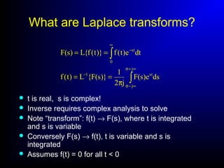
6. Evaluating F(s)=L{f(t)}- Hard Way
remember ∫ ∫−= vduuvudv
)tcos(v,dt)tsin(dv
dtsedu,eu stst
−==
−== −−
∫
∫ ∫
∞
−−
∞ ∞
−∞−−
−−
=−−=∴
0
stst
0 0
st
0
stst
dt)tcos(es)1(e
dt)tcos(es)tcos(e[dt)tsin(e ]
)tsin(v,dt)tcos(dv
dtsedu,eu stst
==
−== −−
∫∫
∫
∞
−−
∞
−∞−
∞
−
+−=+−
=∴
0
stst
0
st
0
st
0
st
dt)tsin(es)0(edt)tsin(es)tsin(e[
dt)tcos(e
]
2
0
st
0
st2
0 0
st2st
s1
1
dt)tsin(e
1dt)tsin(e)s1(
dt)tsin(es1dt)tsin(se
+
=
=+
=−=
∫
∫
∫ ∫
∞
−
∞
−
∞ ∞
−−
let
let
Substituting, we get:
It only gets worse…

7. Evaluating F(s) = L{f(t)}
This is the easy way ...
Recognize a few different transforms
See table 2.3 on page 42 in textbook
Or see handout ....
Learn a few different properties
Do a little math

8. Table of selected Laplace
Transforms
1s
1
)s(F)t(u)tsin()t(f
1s
s
)s(F)t(u)tcos()t(f
as
1
)s(F)t(ue)t(f
s
1
)s(F)t(u)t(f
2
2
at
+
=⇔=
+
=⇔=
+
=⇔=
=⇔=
−

9. More transforms
1n
n
s
!n
)s(F)t(ut)t(f +
=⇔=
66
5
2
1
s
120
s
!5
)s(F)t(ut)t(f,5n
s
!1
)s(F)t(tu)t(f,1n
s
1
s
!0
)s(F)t(u)t(f,0n
==⇔==
=⇔==
==⇔==
1)s(F)t()t(f =⇔δ=

10. Note on step functions in Laplace
∫
∞
−
=
0
st
dte)t(f)}t(f{L
0t,0)t(u
0t,1)t(u
<=
≥=
Unit step function definition:
Used in conjunction with f(t) → f(t)u(t)
because of Laplace integral limits:

11. Properties of Laplace Transforms
Linearity
Scaling in time
Time shift
“frequency” or s-plane shift
Multiplication by tn
Integration
Differentiation

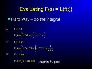
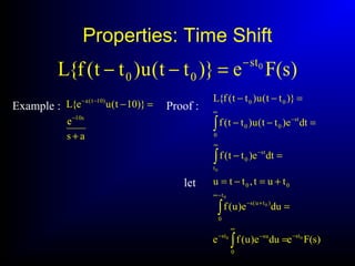
12. Properties: Linearity
)s(Fc)s(Fc)}t(fc)t(fc{L 22112211 +=+
Example :
1s
1
)
1s
)1s()1s(
(
2
1
)
1s
1
1s
1
(
2
1
}e{L
2
1
}e{L
2
1
}e
2
1
e
2
1
{y
)}t{sinh(L
22
tt
tt
−
=
−
−−+
=
+
−
−
=−
=−
=
−
−
Proof :
)s(Fc)s(Fc
dte)t(fcdte)t(fc
dte)]t(fc)t(fc[
)}t(fc)t(fc{L
2211
0
st
22
0
st
11
st
22
0
11
2211
+
=+
=+
=+
∫∫
∫
∞
−
∞
−
−
∞

13. )
a
s
(F
a
1
)}at(f{L =
Example :
22
22
2
2
s
)
s
(
1
)1
)s(
1
(
1
)}t{sin(L
ω+
ω
=
ω+
ω
ω
=+
ω
ω
ω Proof :
)
a
s
(F
a
1
due)u(f
a
1
du
a
1
dt,
a
u
t,atu
dte)at(f
)}at(f{L
a
0
u)
a
s
(
0
st
∫
∫
∞
−
∞
−
=
===
=
=
let
Properties: Scaling in Time

14. Properties: Time Shift
)s(Fe)}tt(u)tt(f{L 0st
00
−
=−−
Example :
as
e
)}10t(ue{L
s10
)10t(a
+
=−
−
−−
Proof :
)s(Fedue)u(fe
due)u(f
tut,ttu
dte)tt(f
dte)tt(u)tt(f
)}tt(u)tt(f{L
00
0
0
0
st
0
sust
t
0
)tu(s
00
t
st
0
0
st
00
00
−
∞
−−
−∞
+−
∞
−
∞
−
∫
∫
∫
∫
=
=
+=−=
=−
=−−
=−−
let

15. Properties: S-plane (frequency)
shift
)as(F)}t(fe{L at
+=−
Example :
22
at
)as(
)}tsin(e{L
ω++
ω
=ω− Proof :
)as(F
dte)t(f
dte)t(fe
)}t(fe{L
0
t)as(
0
stat
at
+
=
=
=
∫
∫
∞
+−
∞
−−
−

16. Properties: Multiplication by tn
)s(F
ds
d
)1()}t(ft{L n
n
nn
−=
Example :
1n
n
n
n
n
s
!n
)
s
1
(
ds
d
)1(
)}t(ut{L
+
=−
=
Proof :
)s(F
s
)1(dte)t(f
s
)1(
dte
s
)t(f)1(
dtet)t(f
dte)t(ft)}t(ft{L
n
n
n
0
st
n
n
n
0
st
n
n
n
0
stn
0
stnn
∂
∂
−=
∂
∂
−
=
∂
∂
−
=
==
∫
∫
∫
∫
∞
−
∞
−
∞
−
∞
−

17. The “D” Operator
1. Differentiation shorthand
2. Integration shorthand
)t(f
dt
d
)t(fD
dt
)t(df
)t(Df
2
2
2
=
=
)t(f)t(Dg
dt)t(f)t(g
t
=
= ∫∞−
)t(fD)t(g
dt)t(f)t(g
1
a
t
a
−
=
= ∫if
then then
if

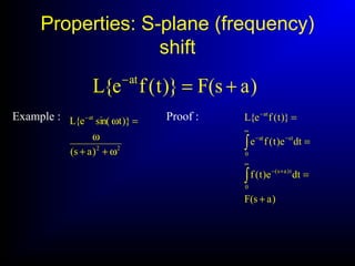
18. Properties: Integrals
s
)s(F
)}t(fD{L 1
0 =−
Example :
)}t{sin(L
1s
1
)
1s
s
)(
s
1
(
)}tcos(D{L
22
1
0
+
=
+
=−
Proof :
let
stst
0
st
1
0
e
s
1
v,dtedv
dt)t(fdu),t(gu
dte)t(g)}t{sin(L
)t(fD)t(g
−−
∞
−
−
−==
==
=
=
∫
∫
∫
=
=+−= −∞−
t
0
st
0
st
dt)t(f)t(g
s
)s(F
dte)t(f
s
1
]e)t(g
s
1
[
∫
∞
−
∞<⇒∞=
0
)()( dtetft st
If t=0, g(t)=0
for so
slower than∫
∞
∞→=
0
)()( tgdttf 0→−st
e

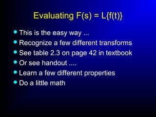
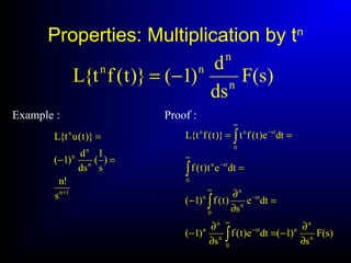
19. Properties: Derivatives
(this is the big one)
)0(f)s(sF)}t(Df{L +
−=
Example :
)}tsin({L
1s
1
1s
)1s(s
1
1s
s
)0(f
1s
s
)}tcos(D{L
2
2
22
2
2
2
2
−=
+
−
+
+−
=−
+
=−
+
=
+
Proof :
)s(sF)0(f
dte)t(fs)]t(fe[
)t(fv,dt)t(f
dt
d
dv
sedu,eu
dte)t(f
dt
d
)}t(Df{L
0
st
0
st
stst
0
st
+−
=+
==
−==
=
+
∞
−∞−
−−
∞
−
∫
∫
let

20. Difference in
The values are only different if f(t) is not
continuous @ t=0
Example of discontinuous function: u(t)
)0(f&)0(f),0(f −+
1)0(u)0(f
1)t(ulim)0(f
0)t(ulim)0(f
0t
0t
==
==
==
+
−
→
+
→
−

21. ?)}t(fD{L 2
=
)0('f)0(sF)s(Fs)0('f))0(f)s(sF(s
)0('f)}t(Df{sL)0(g)s(sG)}t(gD{L
)0('f)0(Df)0(g),t(Df)t(g
2
2
−−=−−=
−=−==
===let
)0(f)0(sf)0('fs)0(fs)s(Fs)}t(fD{L )'1n()'2n()2n()1n(nn −−−−
−−−−−= 
NOTE: to take
you need the value @ t=0 for
called initial conditions!
We will use this to solve differential equations!
→−−
)t(f),t(Df),...t(fD),t(fD 2n1n
)}t(fD{L n
Properties: Nth order derivatives

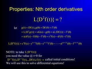
22. Properties: Nth order derivatives
)0(f)s(sF)}t(Df{L −=
)}t(fD{L 2
)0(f)s(sF)}t(Df{L)}t(g{L)s(G
)0('f)0(g
)t(Df)t(g
)0(g)s(sG)}t(Dg{L
)t(fD)t(Dgand)t(Df)t(g 2
−===
=∴
=
−=
==
)0('f)0(sf)s(Fs)0('f)]0(f)s(sF[s)0(g)s(sG)}t(Dg{L 2
−−=−−=−=∴
.etc),t(fD),t(fD 43
Start with
Now apply again
let
then
remember
Can repeat for
)0(f)0(sf)0('fs)0(fs)s(Fs)}t(fD{L )'1n()'2n()2n()1n(nn −−−−
−−−−−= 

23. Relevant Book Sections
Modeling - 2.2
Linear Systems - 2.3, page 38 only
Laplace - 2.4
Transfer functions – 2.5 thru ex 2.4