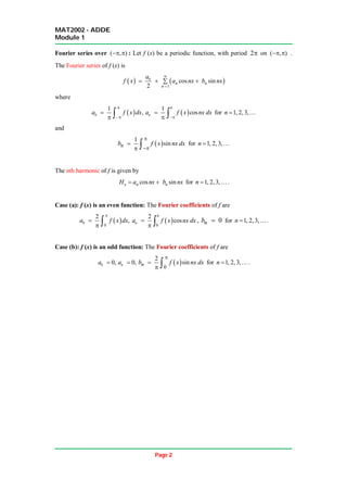
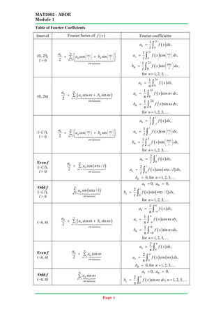
Elementary Concepts of Fourier Series and
Table of Fourier Coefficients
MAT2002 - ADDE
Module 1
Page 1
Fourier series over a general interval: Let f (x) be a periodic function, with period 2l
satisfying the following Dirichlet conditions on each interval (–l, l):
(a) )
(x
f has only a finitely many finite discontinuities;
(b) )
(x
f has only at most finite number of maxima or minima.
Then )
(x
f can be represented by the Fourier series
  0
1
cos sin ,
2
n n
n
a n x n x
f x a b
l l

  
 
   
  
    
 
   
 
where
 
0
1
,
l
l
a f x dx
l 
   
1
cos
n
l
l
n x
a f x dx
l l


 
  
 
 for 1, 2, 3,
n  
and
 
1
sin
l
n
l
n x
b f x dx
l l


 
  
 
 for 1, 2, 3,
n  .
are called the Fourier coefficients of f.
 At a point of finite discontinuity: If f is discontinuous at some interior point c of
(–l, l), then the Fourier series converges to the average
( 0) ( 0)
2
f c f c
  
of left
hand and the right hand limits of f at c
 At the end points: The Fourier series converges to the average
( 0) ( 0)
2
f l f l
   
of left hand limit of f at the right end point l and the right hand limit of f at the left end
point
The nth harmonic of f is given by
cos sin
n n n
n x n x
H a b
l l
 
   
 
   
   
for 1, 2, 3,
n  .
Case (a): f (x) is an even function: The Fourier coefficients of f are
 
0
0
2
,
l
a f x dx
l
   
0
2
cos
n
l n x
a f x dx
l l

 
  
 
 , 0
n
b  for 1, 2, 3,
n  
Case (b): f (x) is an odd function: The Fourier coefficients of f are
0 0,
a  0,
n
a   
0
2
sin
l
n
n x
b f x dx
l l

 
  
 
 for 1, 2, 3,
n  .
MAT2002 - ADDE
Module 1
Page 2
Fourier series over ( , )
  : Let f (x) be a periodic function, with period 2 on ( , )
  .
The Fourier series of f (x) is
   
0
1
cos sin
2
n n
n
a
f x a nx b nx


  

where
 
0
1
,
a f x dx



   
1
cos
n
a f x nx dx



  for 1, 2, 3,
n  
and
 
1
sin
n
b f x nx dx



  for 1, 2, 3,
n  
The nth harmonic of f is given by
cos sin
n n n
H a nx b nx
  for 1, 2, 3,
n  .
Case (a): f (x) is an even function: The Fourier coefficients of f are
 
0
0
2
,
a f x dx


   
0
2
cos
n
a f x nx dx


  , 0
n
b  for 1, 2, 3,
n  .
Case (b): f (x) is an odd function: The Fourier coefficients of f are
0 0,
a  0,
n
a   
0
2
sin
n
b f x nx dx


  for 1, 2, 3,
n  .
MAT2002 - ADDE
Module 1
Page 1
Table of Fourier Coefficients
Interval Fourier Series of ( )
f x Fourier coefficients
(0, 2l),
l > 0
0
th harmonic
1
cos sin
2
n x n x
l l
n
n n
n
a
a b
   
π π
   
   
=
∞
 
+ +
∑  



( )
0
2
0
1
,
l
a f x dx
l
= ∫
( )
2
0
1
cos ,
n x
n l
l
a f x dx
l
 
π
 
 
= ∫
( )
2
0
1
sin ,
n x
l
l
n
b f x dx
l
π
 
 
 
= ∫
for 1, 2, 3,
n = 
(0, 2π) ( )
0
th harmonic
1
cos sin
2
n
n n
n
a
a nx b nx
=
∞
+ +
∑

( )
0
2π
0
1
,
π
a f x dx
= ∫
( )
2π
0
1
cos ,
π
n
a f x nx dx
= ∫
( )
2π
0
1
sin ,
π
n
b f x nxdx
= ∫
for 1, 2, 3,
n = 
(–l, l),
l > 0
0
th harmonic
1
cos sin
2
n x n x
l l
n
n n
n
a
a b
   
π π
   
   
=
∞
 
+ +
∑  



( )
0
1
,
l
l
a f x dx
l −
= ∫
( )
1
cos ,
n x
n l
l
l
a f x dx
l
 
π
 
 
−
= ∫
( )
1
sin ,
n x
l
l
n
l
b f x dx
l
π
 
 
 
−
= ∫
for 1, 2, 3,
n = 
Even f
(–l, l),
l > 0
( )
0
th harmonic
1
cos /
2
n
n
n
a
a n x l
=
∞
+ π
∑




( )
0
0
2
,
l
a f x dx
l
= ∫
( ) ( )
0
2
cos / ,
n
l
a f x n x l dx
l
= π
∫
0,
n
b = for 1, 2, 3,
n = 
Odd f
(–l, l),
l > 0
( )
th harmonic
1
sin /
n
n
n
a n x l
=
∞
π
∑




0 0,
a = 0,
n
a =
( ) ( )
0
2
sin / ,
n
l
b f x n x l dx
l
= π
∫
for 1, 2, 3,
n = 
(–π, π) ( )
0
th harmonic
1
cos sin
2
n
n n
n
a
a nx b nx
=
∞
+ +
∑

( )
0
π
π
1
,
π
a f x dx
−
= ∫
( )
π
π
1
cos ,
π
n
a f x nx dx
−
= ∫
( )
π
π
1
sin ,
π
n
b f x nxdx
−
= ∫
for 1, 2, 3,
n = 
Even f
(–π, π)
0
th harmonic
1
cos
2
n
n
n
a
a nx
=
∞
+ ∑ 



( )
0
π
0
2
,
π
a f x dx
= ∫
( ) ( )
π
0
2
cos ,
π
n
a f x nx dx
= ∫
0,
n
b = for 1, 2, 3,
n = 
Odd f
(–π, π) th harmonic
1
sin
n
n
n
a nx
=
∞
∑ 



0 0,
a = 0,
n
a =
( )
0
2
sin ,
n
b f x nx dx
π
=
π ∫ 1, 2, 3,
n = 
MAT2002 - ADDE
Module 1
Page 2
Formulas frequently used in computing the Fourier coefficients:
1. Leibnitz rule of integration:
a. Version 1 d d
U V UV V U
= −
∫ ∫
:
b. Version 2 1 2 3 4
d ' '' ''' ,
UV x UV U V U V U V
= − + − + ⋅⋅⋅
∫
: where ', '', ''',
U U U ⋅⋅⋅
are the successive derivatives of U, and 1 2 3 4
, , , ,
V V V V ⋅⋅⋅ are the successive
integrals of V
2.
( )
0
2 , if is even
( )
0, if is even
a
f x dx f
f x
f


= 


∫
3. cos
sin px
p
px dx = −
∫ , sin
cos px
p
px dx =
∫
4. [ ]
2 2
sin sin cos
Ax
Ax e
A B
e Bx dx A Bx B Bx
+
= −
∫ ,
5. [ ]
2 2
cos cos sin
Ax
Ax e
A B
e Bx dx A Bx B Bx
+
= +
∫
6. Property of Absolute value function:
x x
= − if 0
x < , x x
= if 0
x >
7. sin0 0,cos0 1 cos2
= = = π
8. sin 0,cos ( 1)n
n n
π = π = − for all n
9. (2 1) 1
2
sin ( 1) , 1,2,3,...
k k
k
− π −
  =
− =
  for all n
10. ( )
2
1, if 1(mod4)
sin
1, if 3(mod4)
n
n
n
π
≡

= 
− ≡

11. ( )
2
cos 0
nπ
= for all odd values of n
12. 1
2
sin cos [sin( ) sin( )]
A B A B A B
⋅ = + + −
13. 1
2
cos sin [sin( ) sin( )]
A B A B A B
⋅ = + − −
14. 1
2
cos cos [cos( ) cos( )]
A B A B A B
⋅ = + + −
15. 1
2
sin sin [cos( ) cos( )]
A B A B A B
⋅ = − − −
16. 1
2
sin cos sin 2
A A A
⋅ =
17. 2 2 2 2
cos2 2cos 1 cos sin 1 2sin
A A A A A
= − = − = −

1.1 Elementary Concepts.pdf

  • 1.
    Elementary Concepts ofFourier Series and Table of Fourier Coefficients
  • 2.
    MAT2002 - ADDE Module1 Page 1 Fourier series over a general interval: Let f (x) be a periodic function, with period 2l satisfying the following Dirichlet conditions on each interval (–l, l): (a) ) (x f has only a finitely many finite discontinuities; (b) ) (x f has only at most finite number of maxima or minima. Then ) (x f can be represented by the Fourier series   0 1 cos sin , 2 n n n a n x n x f x a b l l                           where   0 1 , l l a f x dx l      1 cos n l l n x a f x dx l l           for 1, 2, 3, n   and   1 sin l n l n x b f x dx l l           for 1, 2, 3, n  . are called the Fourier coefficients of f.  At a point of finite discontinuity: If f is discontinuous at some interior point c of (–l, l), then the Fourier series converges to the average ( 0) ( 0) 2 f c f c    of left hand and the right hand limits of f at c  At the end points: The Fourier series converges to the average ( 0) ( 0) 2 f l f l     of left hand limit of f at the right end point l and the right hand limit of f at the left end point The nth harmonic of f is given by cos sin n n n n x n x H a b l l                 for 1, 2, 3, n  . Case (a): f (x) is an even function: The Fourier coefficients of f are   0 0 2 , l a f x dx l     0 2 cos n l n x a f x dx l l          , 0 n b  for 1, 2, 3, n   Case (b): f (x) is an odd function: The Fourier coefficients of f are 0 0, a  0, n a    0 2 sin l n n x b f x dx l l          for 1, 2, 3, n  .
  • 3.
    MAT2002 - ADDE Module1 Page 2 Fourier series over ( , )   : Let f (x) be a periodic function, with period 2 on ( , )   . The Fourier series of f (x) is     0 1 cos sin 2 n n n a f x a nx b nx       where   0 1 , a f x dx        1 cos n a f x nx dx      for 1, 2, 3, n   and   1 sin n b f x nx dx      for 1, 2, 3, n   The nth harmonic of f is given by cos sin n n n H a nx b nx   for 1, 2, 3, n  . Case (a): f (x) is an even function: The Fourier coefficients of f are   0 0 2 , a f x dx       0 2 cos n a f x nx dx     , 0 n b  for 1, 2, 3, n  . Case (b): f (x) is an odd function: The Fourier coefficients of f are 0 0, a  0, n a    0 2 sin n b f x nx dx     for 1, 2, 3, n  .
  • 4.
    MAT2002 - ADDE Module1 Page 1 Table of Fourier Coefficients Interval Fourier Series of ( ) f x Fourier coefficients (0, 2l), l > 0 0 th harmonic 1 cos sin 2 n x n x l l n n n n a a b     π π         = ∞   + + ∑      ( ) 0 2 0 1 , l a f x dx l = ∫ ( ) 2 0 1 cos , n x n l l a f x dx l   π     = ∫ ( ) 2 0 1 sin , n x l l n b f x dx l π       = ∫ for 1, 2, 3, n =  (0, 2π) ( ) 0 th harmonic 1 cos sin 2 n n n n a a nx b nx = ∞ + + ∑  ( ) 0 2π 0 1 , π a f x dx = ∫ ( ) 2π 0 1 cos , π n a f x nx dx = ∫ ( ) 2π 0 1 sin , π n b f x nxdx = ∫ for 1, 2, 3, n =  (–l, l), l > 0 0 th harmonic 1 cos sin 2 n x n x l l n n n n a a b     π π         = ∞   + + ∑      ( ) 0 1 , l l a f x dx l − = ∫ ( ) 1 cos , n x n l l l a f x dx l   π     − = ∫ ( ) 1 sin , n x l l n l b f x dx l π       − = ∫ for 1, 2, 3, n =  Even f (–l, l), l > 0 ( ) 0 th harmonic 1 cos / 2 n n n a a n x l = ∞ + π ∑     ( ) 0 0 2 , l a f x dx l = ∫ ( ) ( ) 0 2 cos / , n l a f x n x l dx l = π ∫ 0, n b = for 1, 2, 3, n =  Odd f (–l, l), l > 0 ( ) th harmonic 1 sin / n n n a n x l = ∞ π ∑     0 0, a = 0, n a = ( ) ( ) 0 2 sin / , n l b f x n x l dx l = π ∫ for 1, 2, 3, n =  (–π, π) ( ) 0 th harmonic 1 cos sin 2 n n n n a a nx b nx = ∞ + + ∑  ( ) 0 π π 1 , π a f x dx − = ∫ ( ) π π 1 cos , π n a f x nx dx − = ∫ ( ) π π 1 sin , π n b f x nxdx − = ∫ for 1, 2, 3, n =  Even f (–π, π) 0 th harmonic 1 cos 2 n n n a a nx = ∞ + ∑     ( ) 0 π 0 2 , π a f x dx = ∫ ( ) ( ) π 0 2 cos , π n a f x nx dx = ∫ 0, n b = for 1, 2, 3, n =  Odd f (–π, π) th harmonic 1 sin n n n a nx = ∞ ∑     0 0, a = 0, n a = ( ) 0 2 sin , n b f x nx dx π = π ∫ 1, 2, 3, n = 
  • 5.
    MAT2002 - ADDE Module1 Page 2 Formulas frequently used in computing the Fourier coefficients: 1. Leibnitz rule of integration: a. Version 1 d d U V UV V U = − ∫ ∫ : b. Version 2 1 2 3 4 d ' '' ''' , UV x UV U V U V U V = − + − + ⋅⋅⋅ ∫ : where ', '', ''', U U U ⋅⋅⋅ are the successive derivatives of U, and 1 2 3 4 , , , , V V V V ⋅⋅⋅ are the successive integrals of V 2. ( ) 0 2 , if is even ( ) 0, if is even a f x dx f f x f   =    ∫ 3. cos sin px p px dx = − ∫ , sin cos px p px dx = ∫ 4. [ ] 2 2 sin sin cos Ax Ax e A B e Bx dx A Bx B Bx + = − ∫ , 5. [ ] 2 2 cos cos sin Ax Ax e A B e Bx dx A Bx B Bx + = + ∫ 6. Property of Absolute value function: x x = − if 0 x < , x x = if 0 x > 7. sin0 0,cos0 1 cos2 = = = π 8. sin 0,cos ( 1)n n n π = π = − for all n 9. (2 1) 1 2 sin ( 1) , 1,2,3,... k k k − π −   = − =   for all n 10. ( ) 2 1, if 1(mod4) sin 1, if 3(mod4) n n n π ≡  =  − ≡  11. ( ) 2 cos 0 nπ = for all odd values of n 12. 1 2 sin cos [sin( ) sin( )] A B A B A B ⋅ = + + − 13. 1 2 cos sin [sin( ) sin( )] A B A B A B ⋅ = + − − 14. 1 2 cos cos [cos( ) cos( )] A B A B A B ⋅ = + + − 15. 1 2 sin sin [cos( ) cos( )] A B A B A B ⋅ = − − − 16. 1 2 sin cos sin 2 A A A ⋅ = 17. 2 2 2 2 cos2 2cos 1 cos sin 1 2sin A A A A A = − = − = −