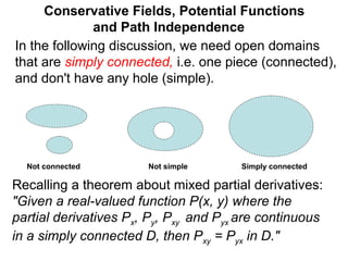
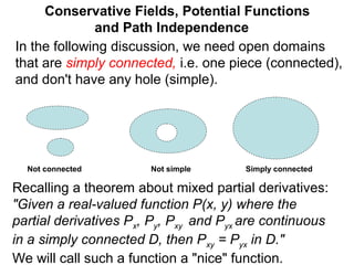
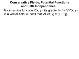
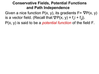
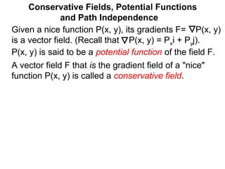
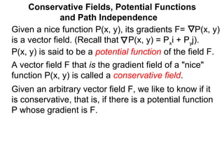
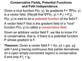
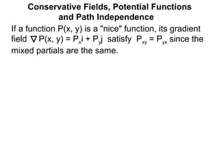
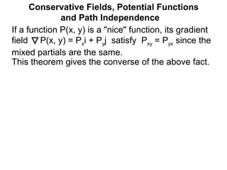
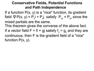
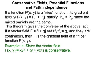
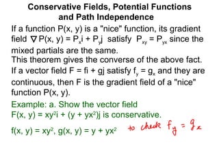
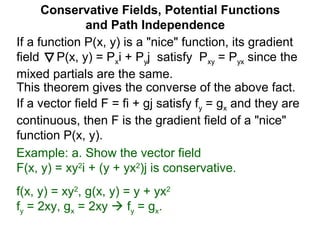
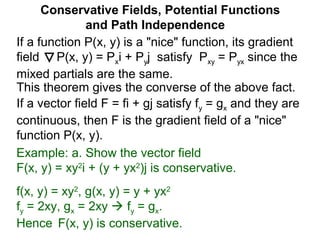
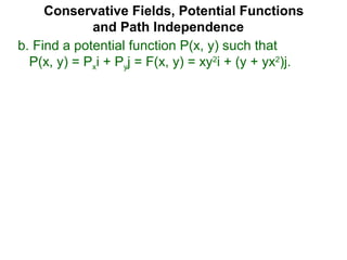
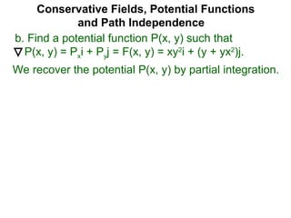
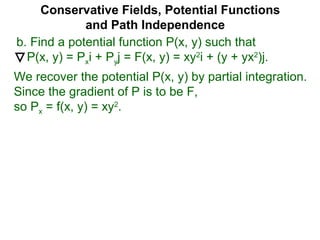
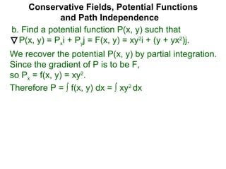
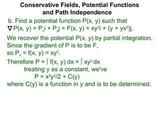
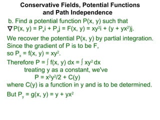
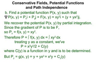
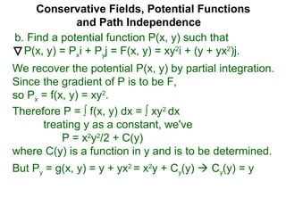
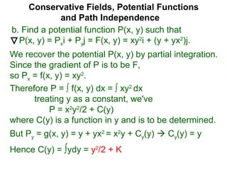
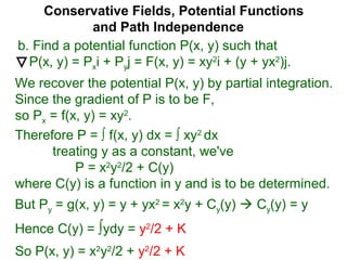
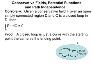
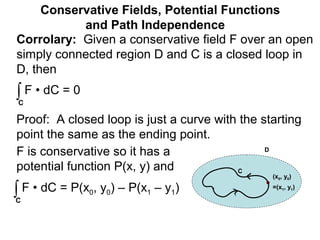
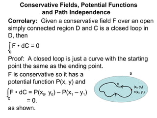
Conservative Fields, Potential Functions
and Path Independence
Conservative Fields, Potential Functions
and Path Independence
In the following discussion, we need open domains
that are simply connected, i.e. one piece (connected),
and don't have any hole (simple).
Conservative Fields, Potential Functions
and Path Independence
In the following discussion, we need open domains
that are simply connected, i.e. one piece (connected),
and don't have any hole (simple).
Not simpleNot connected Simply connected
Conservative Fields, Potential Functions
and Path Independence
In the following discussion, we need open domains
that are simply connected, i.e. one piece (connected),
and don't have any hole (simple).
Not simpleNot connected Simply connected
Recalling a theorem about mixed partial derivatives:
"Given a real-valued function P(x, y) where the
partial derivatives Px, Py, Pxy and Pyx are continuous
in a simply connected D, then Pxy = Pyx in D."
We will call such a function a "nice" function.
Conservative Fields, Potential Functions
and Path Independence
Given a nice function P(x, y), its gradients F= P(x, y)
is a vector field.
Conservative Fields, Potential Functions
and Path Independence
Given a nice function P(x, y), its gradients F= P(x, y)
is a vector field. (Recall that P(x, y) = fxi + fyj).
Given a nice function P(x, y), its gradients F= P(x, y)
is a vector field. (Recall that P(x, y) = fxi + fyj).
P(x, y) is said to be a potential function of the field F.
Conservative Fields, Potential Functions
and Path Independence
Given a nice function P(x, y), its gradients F= P(x, y)
is a vector field. (Recall that P(x, y) = Pxi + Pyj).
P(x, y) is said to be a potential function of the field F.
Conservative Fields, Potential Functions
and Path Independence
A vector field F that is the gradient field of a "nice"
function P(x, y) is called a conservative field.
Conservative Fields, Potential Functions
and Path Independence
A vector field F that is the gradient field of a "nice"
function P(x, y) is called a conservative field.
Given an arbitrary vector field F, we like to know if it
is conservative, that is, if there is a potential function
P whose gradient is F.
Given a nice function P(x, y), its gradients F= P(x, y)
is a vector field. (Recall that P(x, y) = Pxi + Pyj).
P(x, y) is said to be a potential function of the field F.
Theorem: Given a vector field F = f(x, y)i + g(x, y)j
with f and g having continuous first partial derivatives
(in a open simply connected region) is conservative
if and only if fy = gx.
Conservative Fields, Potential Functions
and Path Independence
A vector field F that is the gradient field of a "nice"
function P(x, y) is called a conservative field.
Given an arbitrary vector field F, we like to know if it
is conservative, that is, if there is a potential function
P whose gradient is F.
Given a nice function P(x, y), its gradients F= P(x, y)
is a vector field. (Recall that P(x, y) = Pxi + Pyj).
P(x, y) is said to be a potential function of the field F.
Conservative Fields, Potential Functions
and Path Independence
If a function P(x, y) is a "nice" function, its gradient
field P(x, y) = Pxi + Pyj satisfy Pxy = Pyx since the
mixed partials are the same.
This theorem gives the converse of the above fact.
Conservative Fields, Potential Functions
and Path Independence
If a function P(x, y) is a "nice" function, its gradient
field P(x, y) = Pxi + Pyj satisfy Pxy = Pyx since the
mixed partials are the same.
This theorem gives the converse of the above fact.
Conservative Fields, Potential Functions
and Path Independence
If a function P(x, y) is a "nice" function, its gradient
field P(x, y) = Pxi + Pyj satisfy Pxy = Pyx since the
mixed partials are the same.
If a vector field F = fi + gj satisfy fy = gx and they are
continuous, then F is the gradient field of a "nice"
function P(x, y).
Example: a. Show the vector field
F(x, y) = xy2
i + (y + yx2
)j is conservative.
f(x, y) = xy2
, g(x, y) = y + yx2
fy = 2xy, gx = 2xy  fy = gx.
Hence F(x, y) is conservative.
Conservative Fields, Potential Functions
and Path Independence
b. Find a potential function P(x, y) such that
P(x, y) = Pxi + Pyj = F(x, y) = xy2
i + (y + yx2
)j.
Conservative Fields, Potential Functions
and Path Independence
b. Find a potential function P(x, y) such that
P(x, y) = Pxi + Pyj = F(x, y) = xy2
i + (y + yx2
)j.
We recover the potential P(x, y) by partial integration.
Conservative Fields, Potential Functions
and Path Independence
b. Find a potential function P(x, y) such that
P(x, y) = Pxi + Pyj = F(x, y) = xy2
i + (y + yx2
)j.
We recover the potential P(x, y) by partial integration.
Since the gradient of P is to be F,
so Px = f(x, y) = xy2
.
Conservative Fields, Potential Functions
and Path Independence
b. Find a potential function P(x, y) such that
P(x, y) = Pxi + Pyj = F(x, y) = xy2
i + (y + yx2
)j.
We recover the potential P(x, y) by partial integration.
Since the gradient of P is to be F,
so Px = f(x, y) = xy2
.
Therefore P = ∫ f(x, y) dx = ∫ xy2
dx
treating y as a constant, we've
P = x2
y2
/2 + C(y)
where C(y) is a function in y and is to be determined.
Conservative Fields, Potential Functions
and Path Independence
b. Find a potential function P(x, y) such that
P(x, y) = Pxi + Pyj = F(x, y) = xy2
i + (y + yx2
)j.
We recover the potential P(x, y) by partial integration.
Since the gradient of P is to be F,
so Px = f(x, y) = xy2
.
But Py = g(x, y) = y + yx2
= x2
y + Cy(y)
Therefore P = ∫ f(x, y) dx = ∫ xy2
dx
treating y as a constant, we've
P = x2
y2
/2 + C(y)
where C(y) is a function in y and is to be determined.
Conservative Fields, Potential Functions
and Path Independence
b. Find a potential function P(x, y) such that
P(x, y) = Pxi + Pyj = F(x, y) = xy2
i + (y + yx2
)j.
We recover the potential P(x, y) by partial integration.
Since the gradient of P is to be F,
so Px = f(x, y) = xy2
.
But Py = g(x, y) = y + yx2
= x2
y + Cy(y)  Cy(y) = y
Hence C(y) = ∫ydy = y2
/2 + K
Therefore P = ∫ f(x, y) dx = ∫ xy2
dx
treating y as a constant, we've
P = x2
y2
/2 + C(y)
where C(y) is a function in y and is to be determined.
So P(x, y) = x2
y2
/2 + y2
/2 + K
Fundemental Theorem of Line Integral
Conservative Fields, Potential Functions
and Path Independence
Fundemental Theorem of Line Integral
Given a conservative field F in a open simply
connected domain D and let P(x, y) be a potential
function of F .
Conservative Fields, Potential Functions
and Path Independence
Fundemental Theorem of Line Integral
Given a conservative field F in a open simply
connected domain D and let P(x, y) be a potential
function of F . Let (x0, y0) and (x1, y1) be two points in
D and C be any continuous curve from (x0, y0) to
(x1, y1).
Conservative Fields, Potential Functions
and Path Independence
(x0, y0)
(x1, y1)C
Fundemental Theorem of Line Integral
Given a conservative field F in a open simply
connected domain D and let P(x, y) be a potential
function of F . Let (x0, y0) and (x1, y1) be two points in
D and C be any continuous curve from (x0, y0) to
(x1, y1). Then the line integral
Conservative Fields, Potential Functions
and Path Independence
∫C
F • dC = P(x1, y1) – P(x0, y0)
(x0, y0)
(x1, y1)C1
C2
C3
From the theorem, the line
integrals in the figure
∫C1
F • dC = ∫C2
F • dC = ∫C3
F • dC
are the same in a conservative field F.
Conservative Fields, Potential Functions
and Path Independence
c. Use the fact that P(x, y) = x2
y2
/2 + y2
/2 + k is the
potential function of F(x, y) = xy2
i + (y + yx2
)j.
Find where
C = <cos(t), sin(t)> with
π/2 < t < π .
∫C
F • dC
Conservative Fields, Potential Functions
and Path Independence
c. Use the fact that P(x, y) = x2
y2
/2 + y2
/2 + k is the
potential function of F(x, y) = xy2
i + (y + yx2
)j.
Find where
C = <cos(t), sin(t)> with
π/2 < t < π .
∫C
F • dC
C (0, 1)
(-1, 0)
Conservative Fields, Potential Functions
and Path Independence
c. Use the fact that P(x, y) = x2
y2
/2 + y2
/2 + k is the
potential function of F(x, y) = xy2
i + (y + yx2
)j.
Find where
C = <cos(t), sin(t)> with
π/2 < t < π .
∫C
F • dC
Since F is conservative with potential P and
C(π/2) = (0, 1), C(π) = (-1, 0) as the starting and
ending points in the domain,
C (0, 1)
(-1, 0)
Conservative Fields, Potential Functions
and Path Independence
c. Use the fact that P(x, y) = x2
y2
/2 + y2
/2 + k is the
potential function of F(x, y) = xy2
i + (y + yx2
)j.
Find where
C = <cos(t), sin(t)> with
π/2 < t < π .
∫C
F • dC
Since F is conservative with potential P and
C(π/2) = (0, 1), C(π) = (-1, 0) as the starting and
ending points in the domain, therefore
∫C
F • dC = P(-1, 0) – P(0, 1)
C (0, 1)
(-1, 0)
Conservative Fields, Potential Functions
and Path Independence
c. Use the fact that P(x, y) = x2
y2
/2 + y2
/2 + k is the
potential function of F(x, y) = xy2
i + (y + yx2
)j.
Find where
C = <cos(t), sin(t)> with
π/2 < t < π .
∫C
F • dC
Since F is conservative with potential P and
C(π/2) = (0, 1), C(π) = (-1, 0) as the starting and
ending points in the domain, therefore
∫C
F • dC = P(-1, 0) – P(0, 1) = 0 – ½
C (0, 1)
(-1, 0)
Conservative Fields, Potential Functions
and Path Independence
c. Use the fact that P(x, y) = x2
y2
/2 + y2
/2 + k is the
potential function of F(x, y) = xy2
i + (y + yx2
)j.
Find where
C = <cos(t), sin(t)> with
π/2 < t < π .
∫C
F • dC
Since F is conservative with potential P and
C(π/2) = (0, 1), C(π) = (-1, 0) as the starting and
ending points in the domain, therefore
∫C
F • dC = P(-1, 0) – P(0, 1) = 0 – ½ = -1/2.
C (0, 1)
(-1, 0)
Corrolary: Given a conservative field F over an open
simply connected region D and C is a closed loop in
D, then
Conservative Fields, Potential Functions
and Path Independence
∫C
F • dC = 0
Corrolary: Given a conservative field F over an open
simply connected region D and C is a closed loop in
D, then
Conservative Fields, Potential Functions
and Path Independence
∫C
F • dC = 0
C
D
Corrolary: Given a conservative field F over an open
simply connected region D and C is a closed loop in
D, then
Conservative Fields, Potential Functions
and Path Independence
∫C
F • dC = 0
(x0, y0)
=(x1, y1)
Proof: A closed loop is just a curve with the starting
point the same as the ending point.
F is conservative so it has a
potential function P(x, y) and
∫C
F • dC = P(x0, y0) – P(x1 – y1)
= 0.
as shown.
C
D

29 conservative fields potential functions

  • 1.
    Conservative Fields, PotentialFunctions and Path Independence
  • 2.
    Conservative Fields, PotentialFunctions and Path Independence In the following discussion, we need open domains that are simply connected, i.e. one piece (connected), and don't have any hole (simple).
  • 3.
    Conservative Fields, PotentialFunctions and Path Independence In the following discussion, we need open domains that are simply connected, i.e. one piece (connected), and don't have any hole (simple). Not simpleNot connected Simply connected
  • 4.
    Conservative Fields, PotentialFunctions and Path Independence In the following discussion, we need open domains that are simply connected, i.e. one piece (connected), and don't have any hole (simple). Not simpleNot connected Simply connected Recalling a theorem about mixed partial derivatives: "Given a real-valued function P(x, y) where the partial derivatives Px, Py, Pxy and Pyx are continuous in a simply connected D, then Pxy = Pyx in D."
  • 5.
    Conservative Fields, PotentialFunctions and Path Independence In the following discussion, we need open domains that are simply connected, i.e. one piece (connected), and don't have any hole (simple). Not simpleNot connected Simply connected Recalling a theorem about mixed partial derivatives: "Given a real-valued function P(x, y) where the partial derivatives Px, Py, Pxy and Pyx are continuous in a simply connected D, then Pxy = Pyx in D." We will call such a function a "nice" function.
  • 6.
    Conservative Fields, PotentialFunctions and Path Independence Given a nice function P(x, y), its gradients F= P(x, y) is a vector field.
  • 7.
    Conservative Fields, PotentialFunctions and Path Independence Given a nice function P(x, y), its gradients F= P(x, y) is a vector field. (Recall that P(x, y) = fxi + fyj).
  • 8.
    Given a nicefunction P(x, y), its gradients F= P(x, y) is a vector field. (Recall that P(x, y) = fxi + fyj). P(x, y) is said to be a potential function of the field F. Conservative Fields, Potential Functions and Path Independence
  • 9.
    Given a nicefunction P(x, y), its gradients F= P(x, y) is a vector field. (Recall that P(x, y) = Pxi + Pyj). P(x, y) is said to be a potential function of the field F. Conservative Fields, Potential Functions and Path Independence A vector field F that is the gradient field of a "nice" function P(x, y) is called a conservative field.
  • 10.
    Conservative Fields, PotentialFunctions and Path Independence A vector field F that is the gradient field of a "nice" function P(x, y) is called a conservative field. Given an arbitrary vector field F, we like to know if it is conservative, that is, if there is a potential function P whose gradient is F. Given a nice function P(x, y), its gradients F= P(x, y) is a vector field. (Recall that P(x, y) = Pxi + Pyj). P(x, y) is said to be a potential function of the field F.
  • 11.
    Theorem: Given avector field F = f(x, y)i + g(x, y)j with f and g having continuous first partial derivatives (in a open simply connected region) is conservative if and only if fy = gx. Conservative Fields, Potential Functions and Path Independence A vector field F that is the gradient field of a "nice" function P(x, y) is called a conservative field. Given an arbitrary vector field F, we like to know if it is conservative, that is, if there is a potential function P whose gradient is F. Given a nice function P(x, y), its gradients F= P(x, y) is a vector field. (Recall that P(x, y) = Pxi + Pyj). P(x, y) is said to be a potential function of the field F.
  • 12.
    Conservative Fields, PotentialFunctions and Path Independence If a function P(x, y) is a "nice" function, its gradient field P(x, y) = Pxi + Pyj satisfy Pxy = Pyx since the mixed partials are the same.
  • 13.
    This theorem givesthe converse of the above fact. Conservative Fields, Potential Functions and Path Independence If a function P(x, y) is a "nice" function, its gradient field P(x, y) = Pxi + Pyj satisfy Pxy = Pyx since the mixed partials are the same.
  • 14.
    This theorem givesthe converse of the above fact. Conservative Fields, Potential Functions and Path Independence If a function P(x, y) is a "nice" function, its gradient field P(x, y) = Pxi + Pyj satisfy Pxy = Pyx since the mixed partials are the same. If a vector field F = fi + gj satisfy fy = gx and they are continuous, then F is the gradient field of a "nice" function P(x, y).
  • 15.
    This theorem givesthe converse of the above fact. Conservative Fields, Potential Functions and Path Independence If a function P(x, y) is a "nice" function, its gradient field P(x, y) = Pxi + Pyj satisfy Pxy = Pyx since the mixed partials are the same. If a vector field F = fi + gj satisfy fy = gx and they are continuous, then F is the gradient field of a "nice" function P(x, y). Example: a. Show the vector field F(x, y) = xy2 i + (y + yx2 )j is conservative.
  • 16.
    This theorem givesthe converse of the above fact. Conservative Fields, Potential Functions and Path Independence If a function P(x, y) is a "nice" function, its gradient field P(x, y) = Pxi + Pyj satisfy Pxy = Pyx since the mixed partials are the same. If a vector field F = fi + gj satisfy fy = gx and they are continuous, then F is the gradient field of a "nice" function P(x, y). Example: a. Show the vector field F(x, y) = xy2 i + (y + yx2 )j is conservative. f(x, y) = xy2 , g(x, y) = y + yx2
  • 17.
    This theorem givesthe converse of the above fact. Conservative Fields, Potential Functions and Path Independence If a function P(x, y) is a "nice" function, its gradient field P(x, y) = Pxi + Pyj satisfy Pxy = Pyx since the mixed partials are the same. If a vector field F = fi + gj satisfy fy = gx and they are continuous, then F is the gradient field of a "nice" function P(x, y). Example: a. Show the vector field F(x, y) = xy2 i + (y + yx2 )j is conservative. f(x, y) = xy2 , g(x, y) = y + yx2 fy = 2xy, gx = 2xy  fy = gx.
  • 18.
    This theorem givesthe converse of the above fact. Conservative Fields, Potential Functions and Path Independence If a function P(x, y) is a "nice" function, its gradient field P(x, y) = Pxi + Pyj satisfy Pxy = Pyx since the mixed partials are the same. If a vector field F = fi + gj satisfy fy = gx and they are continuous, then F is the gradient field of a "nice" function P(x, y). Example: a. Show the vector field F(x, y) = xy2 i + (y + yx2 )j is conservative. f(x, y) = xy2 , g(x, y) = y + yx2 fy = 2xy, gx = 2xy  fy = gx. Hence F(x, y) is conservative.
  • 19.
    Conservative Fields, PotentialFunctions and Path Independence b. Find a potential function P(x, y) such that P(x, y) = Pxi + Pyj = F(x, y) = xy2 i + (y + yx2 )j.
  • 20.
    Conservative Fields, PotentialFunctions and Path Independence b. Find a potential function P(x, y) such that P(x, y) = Pxi + Pyj = F(x, y) = xy2 i + (y + yx2 )j. We recover the potential P(x, y) by partial integration.
  • 21.
    Conservative Fields, PotentialFunctions and Path Independence b. Find a potential function P(x, y) such that P(x, y) = Pxi + Pyj = F(x, y) = xy2 i + (y + yx2 )j. We recover the potential P(x, y) by partial integration. Since the gradient of P is to be F, so Px = f(x, y) = xy2 .
  • 22.
    Conservative Fields, PotentialFunctions and Path Independence b. Find a potential function P(x, y) such that P(x, y) = Pxi + Pyj = F(x, y) = xy2 i + (y + yx2 )j. We recover the potential P(x, y) by partial integration. Since the gradient of P is to be F, so Px = f(x, y) = xy2 . Therefore P = ∫ f(x, y) dx = ∫ xy2 dx
  • 23.
    Conservative Fields, PotentialFunctions and Path Independence b. Find a potential function P(x, y) such that P(x, y) = Pxi + Pyj = F(x, y) = xy2 i + (y + yx2 )j. We recover the potential P(x, y) by partial integration. Since the gradient of P is to be F, so Px = f(x, y) = xy2 . Therefore P = ∫ f(x, y) dx = ∫ xy2 dx treating y as a constant, we've P = x2 y2 /2 + C(y) where C(y) is a function in y and is to be determined.
  • 24.
    Conservative Fields, PotentialFunctions and Path Independence b. Find a potential function P(x, y) such that P(x, y) = Pxi + Pyj = F(x, y) = xy2 i + (y + yx2 )j. We recover the potential P(x, y) by partial integration. Since the gradient of P is to be F, so Px = f(x, y) = xy2 . But Py = g(x, y) = y + yx2 Therefore P = ∫ f(x, y) dx = ∫ xy2 dx treating y as a constant, we've P = x2 y2 /2 + C(y) where C(y) is a function in y and is to be determined.
  • 25.
    Conservative Fields, PotentialFunctions and Path Independence b. Find a potential function P(x, y) such that P(x, y) = Pxi + Pyj = F(x, y) = xy2 i + (y + yx2 )j. We recover the potential P(x, y) by partial integration. Since the gradient of P is to be F, so Px = f(x, y) = xy2 . But Py = g(x, y) = y + yx2 = x2 y + Cy(y) Therefore P = ∫ f(x, y) dx = ∫ xy2 dx treating y as a constant, we've P = x2 y2 /2 + C(y) where C(y) is a function in y and is to be determined.
  • 26.
    Conservative Fields, PotentialFunctions and Path Independence b. Find a potential function P(x, y) such that P(x, y) = Pxi + Pyj = F(x, y) = xy2 i + (y + yx2 )j. We recover the potential P(x, y) by partial integration. Since the gradient of P is to be F, so Px = f(x, y) = xy2 . But Py = g(x, y) = y + yx2 = x2 y + Cy(y)  Cy(y) = y Therefore P = ∫ f(x, y) dx = ∫ xy2 dx treating y as a constant, we've P = x2 y2 /2 + C(y) where C(y) is a function in y and is to be determined.
  • 27.
    Conservative Fields, PotentialFunctions and Path Independence b. Find a potential function P(x, y) such that P(x, y) = Pxi + Pyj = F(x, y) = xy2 i + (y + yx2 )j. We recover the potential P(x, y) by partial integration. Since the gradient of P is to be F, so Px = f(x, y) = xy2 . But Py = g(x, y) = y + yx2 = x2 y + Cy(y)  Cy(y) = y Hence C(y) = ∫ydy = y2 /2 + K Therefore P = ∫ f(x, y) dx = ∫ xy2 dx treating y as a constant, we've P = x2 y2 /2 + C(y) where C(y) is a function in y and is to be determined.
  • 28.
    Conservative Fields, PotentialFunctions and Path Independence b. Find a potential function P(x, y) such that P(x, y) = Pxi + Pyj = F(x, y) = xy2 i + (y + yx2 )j. We recover the potential P(x, y) by partial integration. Since the gradient of P is to be F, so Px = f(x, y) = xy2 . But Py = g(x, y) = y + yx2 = x2 y + Cy(y)  Cy(y) = y Hence C(y) = ∫ydy = y2 /2 + K Therefore P = ∫ f(x, y) dx = ∫ xy2 dx treating y as a constant, we've P = x2 y2 /2 + C(y) where C(y) is a function in y and is to be determined. So P(x, y) = x2 y2 /2 + y2 /2 + K
  • 29.
    Fundemental Theorem ofLine Integral Conservative Fields, Potential Functions and Path Independence
  • 30.
    Fundemental Theorem ofLine Integral Given a conservative field F in a open simply connected domain D and let P(x, y) be a potential function of F . Conservative Fields, Potential Functions and Path Independence
  • 31.
    Fundemental Theorem ofLine Integral Given a conservative field F in a open simply connected domain D and let P(x, y) be a potential function of F . Let (x0, y0) and (x1, y1) be two points in D and C be any continuous curve from (x0, y0) to (x1, y1). Conservative Fields, Potential Functions and Path Independence
  • 32.
    Fundemental Theorem ofLine Integral Given a conservative field F in a open simply connected domain D and let P(x, y) be a potential function of F . Let (x0, y0) and (x1, y1) be two points in D and C be any continuous curve from (x0, y0) to (x1, y1). Conservative Fields, Potential Functions and Path Independence (x0, y0) (x1, y1)C
  • 33.
    Fundemental Theorem ofLine Integral Given a conservative field F in a open simply connected domain D and let P(x, y) be a potential function of F . Let (x0, y0) and (x1, y1) be two points in D and C be any continuous curve from (x0, y0) to (x1, y1). Then the line integral Conservative Fields, Potential Functions and Path Independence ∫C F • dC = P(x1, y1) – P(x0, y0) (x0, y0) (x1, y1)C
  • 34.
    Fundemental Theorem ofLine Integral Given a conservative field F in a open simply connected domain D and let P(x, y) be a potential function of F . Let (x0, y0) and (x1, y1) be two points in D and C be any continuous curve from (x0, y0) to (x1, y1). Then the line integral Conservative Fields, Potential Functions and Path Independence ∫C F • dC = P(x1, y1) – P(x0, y0) (x0, y0) (x1, y1)C1 C2 C3 From the theorem, the line integrals in the figure ∫C1 F • dC = ∫C2 F • dC = ∫C3 F • dC are the same in a conservative field F.
  • 35.
    Conservative Fields, PotentialFunctions and Path Independence c. Use the fact that P(x, y) = x2 y2 /2 + y2 /2 + k is the potential function of F(x, y) = xy2 i + (y + yx2 )j. Find where C = <cos(t), sin(t)> with π/2 < t < π . ∫C F • dC
  • 36.
    Conservative Fields, PotentialFunctions and Path Independence c. Use the fact that P(x, y) = x2 y2 /2 + y2 /2 + k is the potential function of F(x, y) = xy2 i + (y + yx2 )j. Find where C = <cos(t), sin(t)> with π/2 < t < π . ∫C F • dC C (0, 1) (-1, 0)
  • 37.
    Conservative Fields, PotentialFunctions and Path Independence c. Use the fact that P(x, y) = x2 y2 /2 + y2 /2 + k is the potential function of F(x, y) = xy2 i + (y + yx2 )j. Find where C = <cos(t), sin(t)> with π/2 < t < π . ∫C F • dC Since F is conservative with potential P and C(π/2) = (0, 1), C(π) = (-1, 0) as the starting and ending points in the domain, C (0, 1) (-1, 0)
  • 38.
    Conservative Fields, PotentialFunctions and Path Independence c. Use the fact that P(x, y) = x2 y2 /2 + y2 /2 + k is the potential function of F(x, y) = xy2 i + (y + yx2 )j. Find where C = <cos(t), sin(t)> with π/2 < t < π . ∫C F • dC Since F is conservative with potential P and C(π/2) = (0, 1), C(π) = (-1, 0) as the starting and ending points in the domain, therefore ∫C F • dC = P(-1, 0) – P(0, 1) C (0, 1) (-1, 0)
  • 39.
    Conservative Fields, PotentialFunctions and Path Independence c. Use the fact that P(x, y) = x2 y2 /2 + y2 /2 + k is the potential function of F(x, y) = xy2 i + (y + yx2 )j. Find where C = <cos(t), sin(t)> with π/2 < t < π . ∫C F • dC Since F is conservative with potential P and C(π/2) = (0, 1), C(π) = (-1, 0) as the starting and ending points in the domain, therefore ∫C F • dC = P(-1, 0) – P(0, 1) = 0 – ½ C (0, 1) (-1, 0)
  • 40.
    Conservative Fields, PotentialFunctions and Path Independence c. Use the fact that P(x, y) = x2 y2 /2 + y2 /2 + k is the potential function of F(x, y) = xy2 i + (y + yx2 )j. Find where C = <cos(t), sin(t)> with π/2 < t < π . ∫C F • dC Since F is conservative with potential P and C(π/2) = (0, 1), C(π) = (-1, 0) as the starting and ending points in the domain, therefore ∫C F • dC = P(-1, 0) – P(0, 1) = 0 – ½ = -1/2. C (0, 1) (-1, 0)
  • 41.
    Corrolary: Given aconservative field F over an open simply connected region D and C is a closed loop in D, then Conservative Fields, Potential Functions and Path Independence ∫C F • dC = 0
  • 42.
    Corrolary: Given aconservative field F over an open simply connected region D and C is a closed loop in D, then Conservative Fields, Potential Functions and Path Independence ∫C F • dC = 0 C D
  • 43.
    Corrolary: Given aconservative field F over an open simply connected region D and C is a closed loop in D, then Conservative Fields, Potential Functions and Path Independence ∫C F • dC = 0 (x0, y0) =(x1, y1) Proof: A closed loop is just a curve with the starting point the same as the ending point. C D
  • 44.
    Corrolary: Given aconservative field F over an open simply connected region D and C is a closed loop in D, then Conservative Fields, Potential Functions and Path Independence ∫C F • dC = 0 (x0, y0) =(x1, y1) Proof: A closed loop is just a curve with the starting point the same as the ending point. F is conservative so it has a potential function P(x, y) and ∫C F • dC = P(x0, y0) – P(x1 – y1) C D
  • 45.
    Corrolary: Given aconservative field F over an open simply connected region D and C is a closed loop in D, then Conservative Fields, Potential Functions and Path Independence ∫C F • dC = 0 (x0, y0) =(x1, y1) Proof: A closed loop is just a curve with the starting point the same as the ending point. F is conservative so it has a potential function P(x, y) and ∫C F • dC = P(x0, y0) – P(x1 – y1) = 0. as shown. C D