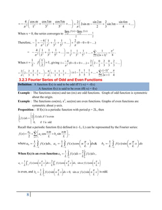
1. The document discusses Fourier series and orthogonal functions. It defines orthogonal functions and provides examples of orthogonal function sets, such as cosine and sine functions. 2. The chief advantage of orthogonal functions is that they allow functions to be represented as generalized Fourier series expansions. The orthogonality of the functions helps determine the Fourier coefficients in a simple way using integrals. 3. Euler's formulae give the expressions for calculating the Fourier coefficients a0, an, and bn of a periodic function f(x) from its values over one period using integrals of f(x) multiplied by cosine and sine terms.

1. 1
UNIT 3
Fourier Series
3.1: ORTHOGONAL FUNCTIONS
Definition: Functions ),...
(
),
( 2
1 x
y
x
y defined on some interval are called orthogonal on a x  b
with respect to the weight function p(x) > 0 if  
b
a
n
m dx
x
y
x
y
x
p 0
)
(
)
(
)
( for m  n.

b
a
n dx
x
y
x
p )
(
)
( 2
is called the square of the norm of )
(x
yn and written as
2
n
y . If the norm is
unity, we say that the set of functions is an orthonormal set. If the weight function is unity, we
simply say that the set is orthogonal on a x  b.
Examples of sequences of orthogonal functions are: The set of functions 1, cos (nx) , n = 1, 2, 3, … or
1, sin(nx) , n = 1, 2, 3, … or 1, cos(nx), sin(nx), n = 1, 2, 3, , on the interval 
2


 a
x
a with
weight functions p(x) = 1 for any real constant a.
The chief advantage of the knowledge of these orthogonal sets of functions is that they yield series
expansions of a given function in a simple fashion. Let 1 2
, ,
y y be an orthogonal set with respect
to the weight function p(x) on an interval b
x
a 
 . Let f(x) be a given function that can be
represented in terms of )
(x
yn by a convergent series,








0
2
2
1
1
0
0 )
(
)
(
)
(
)
(
)
(
m
m
m x
y
a
x
y
a
x
y
a
x
y
a
x
f 
This is called an orthogonal expansion or the generalized Fourier series. The orthogonality of the
functions helps us to find the unknown coefficients 
2
1
0 ,
, a
a
a in a simple fashion. These are
called Fourier coefficients of f(x) with respect to 
,
,
, 2
1
0 y
y
y . If we multiply both side of the above
expansion by p(x)yn(x) for a fixed n, and then integrate over a  x  b, we obtain, assuming term by
term integration is permissible,
dx
x
y
x
y
a
x
p
dx
x
y
x
f
x
p n
b
a
b
a m
m
m
n )
(
)
(
)
(
)
(
)
(
)
(
0
   








dx
x
y
x
p
a
x
y
x
y
x
p
a
m
b
a
b
a
n
n
n
m
m )
(
)
(
)
(
)
(
)
(
0
2
  




2
)
(x
y
a n
n
 , all other
integrals being zero in the right hand side, because of the orthogonality of the set.

2. 2
Thus 2
)
(
)
(
)
(
)
(
x
y
dx
x
y
x
f
x
p
a
n
b
a
n
n

 .
Definition: A function f is said to be a periodic function with period p if p is the least positive number
such that f(x +p) = f(x) for all x in the domain of f. It follows that f(x+np) = f(x) for all x in the
domain of f and all integers n.
Example : f(x) = sinx and g(x) = cos x are the familiar periodic functions with period p = 2.
The constant function h(x) = c is a periodic function, since h(x +p) =c = h(x) for all p (0, ).
Proposition: If f and g are periodic functions with period p, then H(x) = af(x) + bg(x), for some
constants a & b, is a periodic function with period p.
Proof: H(x+p) = a f(x+p) +bg(x +b) = af(x) + bg(x) = H(x) since f(x+p) = f(x) &g(x+p) = g(x)
Therefore, H(x) is a periodic function with period p.
Definition : A functional series of the form
...
sin
cos
2
sin
2
cos
sin
cos
2
2
2
1
1
0







 nx
b
nx
a
x
b
x
a
x
b
x
a
a
n
n

=  





1
0
sin
cos
2 n
n
n nx
b
nx
a
a
is called a trigonometric series; where n
n b
a
a ,
,
0 (n = 1, 2, 3, 
are real constants,) are called the coefficients of the trigonometric series.
If the series converges, say to a function f(x), i.e, 





1
0
)
(
)
sin
cos
(
2 n
n
n x
f
nx
b
nx
a
a
Then f is a period function with period p = 2 , by the above proposition.
Thus f(x+2) = f(x) for all x in the domain of f, where  






1
0
sin
cos
2
)
(
n
n
n nx
b
nx
a
a
x
f .
3.2 Fourier Series
3.2.1 Fourier Series of function with period
Definition : The Fourier series for the periodic function f(x) in an interval α < x < α + 2 is given by.
 






1
0
sin
cos
2
)
(
n
n
n nx
b
nx
a
a
x
f And the coefficients
,
,
0 n
n b
and
a
a n = 1, 2, 3,  are called the Fourier coefficients.
To evaluate the Fourier Coefficients, the following integrals, involving sine and cosine functions are
useful.
i)
2 2
cos sin 0
nxdx nx
   
 
 
 
  , n = 1, 2, 3, 

3. 3
ii)
2 2
1
cos cos [cos( ) cos( ) ]
2
mx nxdx m n x m n x dx
   
 
 
   
 
2
1 1 1
sin( ) sin( )
2
m n x m n x
m n m n
 


 
   
 
 
 
= 0, m  n.
iii)
2
cos sin 0
mx nxdx
 




iv)
2 2
2 2
cos ( ) sin ( ) , 0
nx dx nx dx n
   
 

 
  
 
2 2
2
2 1 cos(2 ) 1 1
cos ( ) sin 2
2 2 2
nx
nx dx dx x x
n
   
 

 
 

  
  
 
 
    
 


 a
a 2
2
1
In addition to these properties of integrals involving sine and cosine functions, we often need the
following trigonometric functions for particular arguments.
i)
n
n
n )
1
(
cos
2
)
1
2
sin( 


 

and (ii) ,
0
2
)
1
2
cos(
sin 



 n
n n = 1, 2, 
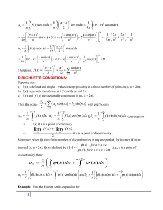
Theorem : (Euler’s Formulae): The Fourier coefficients in
 






1
0
sin
cos
2
)
(
n
n
n nx
b
nx
a
a
x
f are given by
2 2
0
1 1
( ) , ( )cos
n
a f x dx a f x nxdx
   
 
 
 
 
  and
2
1
( )sin
n
b f x nxdx
 



 
Corollary : 1. If  = 0, the interval becomes 0 < x < 2 , and Euler’s formulae are given by:




2
0
0 )
(
1
dx
x
f
a , 



2
0
cos
)
(
1
nxdx
x
f
an
, 



2
0
sin
)
(
1
nxdx
x
f
bn .
2. If  = - , then the interval becomes -< x < , and the Euler’s Formulae and given by:






dx
x
f
a )
(
1
0 , 





nxdx
x
f
a cos
)
(
1
0 , 





nxdx
x
f
bn sin
)
(
1
.
Examples If
2
2
)
( 




 

x
x
f

in the range (0, 2), show that 




1
2
2
cos
12
)
(
n n
nx
x
f

.
Solution: The Fourier serves for f in (0, 2) is  






1
0
sin
cos
2
)
(
n
n
n nx
b
nx
a
a
x
f , where


 







 












2
0
2
2
2
2
2
0
0 )
2
(
4
1
2
1
)
(
1
dx
x
x
dx
x
dx
x
f
a
6
3
1
4
1 2
2
0
3
2
2 













 x
x
x

4. 4


 






 










2
0
2
2
2
0
2
0
)
cos
)
(
4
1
cos
2
1
cos
)
(
1
nxdx
x
nxdx
x
nxdx
x
f
an




2
0
3
2
2
)
sin(
(
2
)
cos(
)
(
2
)
sin(
)
(
4
1





 






 




n
nx
n
nx
x
nx
n
x
= 2
2
2
1
2
2
4
1
n
n
n











dx
nx
x
dx
nx
x
f
bn )
sin(
2
1
)
sin(
)
(
1
2
2
0
2
0

 




 







0
)
cos(
2
)
sin(
)
(
2
)
cos(
)
(
4
1
2
0
3
2
2
2













 







 






nx
n
n
nx
x
n
nx
x
Therefore, 









 

1
2
2
2
)
cos(
12
2
)
(
n n
nx
x
x
f


DIRICHLET’S CONDITIONS:
Suppose that:
a) f(x) is defined and single – valued except possibly at a finite number of points in(α, α + 2).
b) f(x) is periodic outside (α, α + 2) with period 2.
c) f(x) and )
(x
f  are sectionally continuous in (α, α + 2).
Then the series 




1
0
)
sin(
)
cos(
(
2 n
n
n nx
b
nx
a
a
with coefficients










2
2
0 )
cos(
)
(
1
,
)
(
1
a
a
a
a
n dx
nx
x
f
a
dx
x
f
a & dx
nx
x
f
b
a
a
n )
sin(
)
(
1
2





converges to
i) f(x) if x is a point of continuity
ii)
2
)
(
)
( lim
lim x
f
x
f
c
x
c
x 




if c is a point of discontinuity .
Moreover, when f(x) has finite number of discontinuities in any one period, for instance if in an
interval (α, α + 2), f(x) is defined by












2
),
(
,
)
(
)
(
a
x
c
for
x
c
x
a
for
x
x
f , i.e., c is a point of
discontinuity, then:
2
0
1
( ) ( )
c a
a c
a x dx x dx

 


 
 
 
 
 
2
0
1
( )cos( ) ( )cos( )
c a
a c
a x nx dx x nx dx

 


 
 
 
 
  and 








  

c
a
a
c
n dx
nx
x
dx
nx
x
b




2
)
sin(
)
(
)
sin(
)
(
1
Example: Find the Fourier series expansion for

5. 5













x
if
x
x
if
x
f
0
,
0
,
)
( and deduce that
8
7
1
5
1
3
1
1
1
)
1
2
(
1 2
2
2
2
2
0
2












n n
.
Solution: Let  
0
1
( ) cos( ) sin( )
2
n n
n
a
f x a nx b nx dx


  

Then 

  



















 0
0
0
0
0
1
1
xdx
dx
xdx
dx
a 





2
1
2
1
2
1
0
2







 x








  

0
0
)
cos(
)
cos(
1




dx
nx
x
dx
nx
an
0 0 0
1 sin( )
cos( ) cos( )
nx
nx dx x nx dx
n

 



   
 
 
 
1
1
1
)
cos(
)
sin(
)
sin(
1
2
0
2
0
0












 
n
n
n
nx
dx
n
nx
n
nx
x






and 







  

0
0
)
sin(
)
sin(
1




dx
nx
x
dx
nx
bn 






  0
0
)
sin(
1
)
sin( dx
nx
x
dx
nx











 

dx
n
nx
n
nx
x
n
nx


  0
0
0
)
cos(
)
cos(
1
)
cos(

















 0
2
)
(
)
1
(
1
)
1
(
1
n
nx
Sin
n
n
n
n
n
n
n
n
n
n 1
1
1
)
1
(
2
1
0
)
1
(
)
1
(
1 











Hence, 










 







1
1
2
)
sin(
)
1
(
2
1
)
cos(
1
)
1
(
2
2
1
)
(
n
n
n
nx
n
nx
n
x
f














 
)
5
(
5
2
)
3
(
3
2
2
4 2
2
x
Cos
x
Cos
Cosx














 
)
5
(
5
3
)
4
(
4
1
)
3
(
)
2
(
2
1
3 x
Sin
x
Sin
x
Sin
x
Sin
Sinx





















 
 )
3
(
)
2
(
2
1
sin
3
5
)
5
(
3
)
3
(
1
2
4 2
2
2
x
Sin
x
Sin
x
x
Cos
x
Cos
Cosx


.
By Dirichlet’s Condition, we have that
 

 



















0
0
5
1
3
1
1
1
2
4
2
)
(
)
(
2
2
2
0
0
lim
lim


x
f
x
f
x
x














 
2
2
2
5
1
3
1
1
1
2
4
2
0



8
2
4
5
1
3
1
1
1
2
4
2
2
2
2































 
8
)
1
2
(
1
;
.
.
5
1
3
1
1
1 2
0
2
2
2
2






 


n n
e
i
 .

6. 6
3.2.2 Fourier Series of Functions with arbitrary period P = 2L
In many engineering problems, the period of the function required to be expanded is not 2 but some
other interval say 2L. In order to apply the foregoing discussion to functions of period 2L, this interval
must be converted to the length 2 . This involves only a proportional change in the scale.
Consider the periodic function f(x) defined on (α, α + 2L). To change the problem to period 2 put
x
L
t

 which implies that t
L
x

 . This gives when )
2
,
( L
a
a
x 
 . Thus the function f(x) of period
2L in (α, α + 2L) is transformed to function 





t
L
f

of period 2 in , 2
L L
 

 

 
 
. Hence 





 t
L
f

can be expressed in Fourier series as:
 













1
0
)
sin(
)
cos(
2
)
(
n
n
n nt
b
nt
a
a
t
L
f
t
g

, where
,
)
cos(
1
,
1
2
2
0 dt
nt
t
L
f
a
dt
t
L
f
a n 






















 



and ,
)
sin(
1
2
dt
nt
t
L
f
bn 










 

where
t
L
x
and
L
a


 
 .
Marking the inverse substitution x
L
t

 and noting that dx
L
dt

 in the above formula, the Fourier
series Expansion of f(x) in the interval (α, α +2L) is given by


























1
0
sin
cos
2
)
(
n
n
n x
L
n
b
x
L
n
a
a
x
f


where
2 2
0
1 1
( ) , ( )cos
L L
n
a f x dx a f x n x dx
L L L
 
 

 
 
   
 
  and
2
1
( )sin
L
n
b f x n x dx
L L




 
  
 

Corollary :
i. Putting α = 0 in these formulae, we get the corresponding Fourier Coefficients for the
interval (0, 2L)
2 2
0
0 0
1 1
( ) , ( )cos
L L
n
a f x dx a f x n x dx
L L L

 
   
 
 
dx
x
L
n
x
f
L
b
L
n  






2
0
sin
)
(
1 

7. 7
ii. Putting a = - L in the above formulae, we get the results:
dx
x
L
n
x
f
L
a
dx
x
f
L
a
L
L
L
L
n
 
 









cos
)
(
1
,
)
(
1
0 and
1
( )sin
L
n
L
b f x n x dx
L L


 
  
 
 are the Fourier coefficients
in the interval (-L, L).
Example : Find the Fourier series of the periodic function f(x) of period 2, where










1
0
,
2
0
1
,
1
)
(
x
for
x
x
for
x
f and show that
4
7
1
5
1
3
1
1
8
7
1
5
1
3
1
1
2
2
2
2











 
 and
Solution: 2L = 2  L = 1, and  






1
0
sin
cos
2
)
(
n
n
n x
n
b
x
n
a
a
x
f 

where
1
1
1 0 1
2
0
1 1 0 0 0
1 1
( ) ( ) 2 1 1 0
1
L
L
a f x dx f x dx dx xdx x x
L

  
          
   
  
 




1
1
0
1
1
0
)
cos(
2
)
cos(
)
cos(
)
(
1
1
dx
x
n
x
dx
x
n
dx
x
n
x
f
an 


 
1
0
2
2
1
0
1
0
)
cos(
2
)
sin(
2
)
sin(
x
n
n
x
n
x
n
n
x
n










   
1
2
2
2
2
2
2
)
1
(
1
2
)
)
1
(
1
(
2
1
)
1
(
2 










 n
n
n
n
n
n 


  
 




1
1
0
1
1
0
)
sin(
2
)
sin(
)
sin(
)
(
1
1
dx
x
n
dx
x
n
dx
x
n
x
f
bn 







 

 

1
0
1
0
0
1
)
cos(
)
cos(
2
)
cos(
dx
x
n
x
n
x
n
n
x
n





 
   
2
0
1 2 sin( )
1 1 1
n n n x
n n n

  
 
     
 
 
 
1
1 ( 1) 2( 1) 1 3( 1) 1 3( 1)
n n n n
n n n
  

       
  
Thus  






1
0
)
sin(
)
cos(
2
)
(
n
n
n x
n
b
x
n
a
a
x
f 

 












 







1
1
2
2
1
)
sin(
)
1
(
3
1
)
cos(
)
1
(
1
2
0
n
n
n
x
n
n
x
n
n




x
x
x
x
x 









3
sin
3
4
3
cos
3
4
2
sin
2
sin
4
cos
4
2
2
2










 )
5
sin(
5
4
)
5
cos(
5
4
4
sin
4
2
2
2
x
x
x 






8. 8










 
2
2
2
2
5
5
cos
3
3
cos
1
cos
4 x
x
x 













 
4
4
sin
3
sin
3
2
2
2
sin
sin
2
2 x
x
x
x





When x = 0, the series converges to
2
1
2
)
(
)
( lim
lim 0
0







x
f
x
f
x
x
Therefore, )
0
0
0
(
2
5
1
3
1
1
1
4
2
1
2
2
2
2

 

















= 








 
2
2
2
2
5
1
3
1
1
1
4
 8
)
1
2
(
1
5
1
3
1
1
1 2
0
2
2
2
2







 


n n
 .
When 1
2
1
,
2
1







 f
x , giving 















 

3
2
3
0
3
2
2
0
2
2
)
0
0
0
(
4
1 2























 

7
1
5
1
3
1
1
4
7
2
5
2
3
2
2
2

 4
1
2
)
1
(
7
1
5
1
3
1
1
0









 


n
n
n

3.2.3 Fourier Series of Odd and Even Functions
Definition: A function f(x) is said to be odd iff f (-x) = -f(x)
A function f(x) is said to be even iff(-x) = f(x)
Example : The functions sin(nx) and tan (nx) are odd functions. Graph of odd function is symmetric
about the origin.
Example : The functions cos(nx), x2
, sec(nx) are even functions. Graphs of even functions are
symmetric about y-axis.
Proposition : If f(x) is a periodic function with period p = 2L, then
 
 





L
L
L
dx
x
f
dx
x
f
odd
is
f
if
0,
even
is
f
if
,
)
(
2
)
(
0
Recall that a periodic function f(x) defined in (- L, L) can be represented by the Fourier series:












1
0
sin
cos
2
)
(
n
n
n
L
x
n
b
L
x
n
a
a
x
f


,
where 0
1 1 1
( ) , ( )cos & ( )sin
L L L
n n
L L L
a f x dx a f x n x dx b f x n x dx
L L L L L
 
  
   
  
   
   
  
When f(x) is an even function x
d
x
f
L
dx
x
f
L
a
L
L
L





0
0 )
(
2
)
(
1
,



















 

x
L
n
x
f
ce
dx
x
L
n
x
f
L
dx
x
L
n
x
f
L
a
L
L
L
n



cos
)
(
sin
,
cos
)
(
2
cos
)
(
1
0
is even, and 












 

x
L
n
x
f
ce
dx
x
L
n
x
f
L
b
L
L
n


sin
)
(
sin
,
0
sin
)
(
1
is odd.

9. 9
Therefore, the Fourier series expansion of a periodic even function f(x) contains only the cosine terms
whose coefficients are 
 







L
L
dx
x
L
n
x
f
L
dx
x
f
L
a
0
n
0 cos
)
(
2
a
and
)
(
2 






















   


x
L
n
dx
x
L
n
x
f
L
dx
x
f
L
x
f
L
n
L


cos
cos
)
(
2
)
(
1
)
(
0 1 0
.
When f(x) is odd function: 0
cos
)
(
1
,
0
)
(
1
0 








 
 

dx
x
L
n
x
f
L
a
dx
x
f
L
a
L
L
L
L
n
 , since 





x
L
n
x
f

cos
)
( is odd,
and dx
x
L
n
x
f
L
b
L
L
n 









sin
)
(
1
dx
x
L
n
x
f
L
L
 






0
sin
)
(
2  , since 





x
L
n
x
f

sin
)
( is even.
Thus, if a period function f(x) is odd, its Fourier series expansion contains only the sine terms, whose
coefficients are
0
2
( )sin
L
n
b f x n x dx
L L

 
  
 
 , so that




















  


x
L
n
dx
x
L
n
x
f
L
x
f
n
ts
Coefficien
L


sin
sin
)
(
2
)
(
1 0



 



 

.
Example: Find a series to represent f(x) = x2
in the interval )
,
( 

 . Deduce the values of i)










2
2
2
1
2
1
3
1
2
1
1
1
)
1
(
n
n
n
=
12
2

and ii)
6
3
1
2
1
1
1
1 2
2
2
2
1
2










n n
Solution: Let f(x) = x2
in the interval )
,
( 

 be represented by Fourier series as
0
1
( ) cos sin
2
n n
n
a n n
f x a x b x
 


 
  
 
 
 . Here )
(
,
.
),
(
)
(
)
( 2
2
x
f
e
i
x
f
x
x
x
f 


 is even in )
,
( 

 .
Therefore,
2
2
0
0 0
2 2 2
( )
3
l l
l
a f x dx x dx
l l
  
 
2
0 0
2 2
( )cos cos
n
n x n
a f x dx x x dx
 
   
 
   
   
 





















 



 0
0
2
sin
2
sin
2
dx
x
n
x
x
n
x
n
























 





0
0
2
2
cos
cos
4
dx
x
n
x
n
x
n



0
)
1
(
4
sin
)
1
(
4
2
2
2
0
2
2



















 n
n
n
b
and
n
x
n
n
n 









Therefore, =
2 2
2
2 2
1
4 ( 1)
( ) cos
3
n
n
n
f x x x
n




  
   
 
 














 





2
2
2
2
2
2
3
3
cos
2
2
cos
1
cos
4
3
x
x
x




,
which is the required Fourier series. i) Putting x = 0, we get 










 


2
2
2
2
2
2
3
1
2
1
1
1
4
3
0
)
0
(

f
i.e,
12
)
1
( 2
1
2
1







n
n
n

10. 10
ii) Putting 

x , we get
2 2 2 2
2
2 2 2 2 2
( )
4 1 1 1 1
2 2 3 1 2 3 4
lim ( )
lim
x x
f x f x

 
 

  
        
 
  



































4
3
2
4
1
3
1
2
1
1
1
4
1
3
1
2
1
1
1
4
3
1
1
2
2
2
2
2
2
2
2
2
2
3
2



 6
1 2
1
2


 


n n
HALF – RANGE EXPANSION
In many problems of physics and engineering there is a practical need to apply a Fourier Series to a
non – periodic function F(x) on the interval 0 < x < T. Because of physical or mathematical
considerations, it may be possible to extend F(x) over the interval –T < x < T, making it periodic of
period P = 2T. The following figures illustrate the odd and even extensions of F(x) which have
Fourier Sine and Fourier Cosine series, respectively.
a) Original function
b) Odd Extension c) Even Extension
Examples : Express f(x) = x as a half – range
a) Sine series in 0 < x < 2.b)Cosine series in 0 < x < 2.
Solutions: The graph of f(x) = x in 0 < x <2 is the line OA. Let us extend the function f(x) in the
interval -2 < x < 0 (shown by the line BO) so that the new function is symmetric about the origin and ,
therefore, represents an odd function in (-2, 2)
y
A
-2
-1
-2 -1 0 1 2
-1
B -2
Hence the Fourier series for f(x) over the full period (-2, 2) will contain only sine series terms given by










1 2
sin
)
(
n
n
x
n
b
x
f
 Where dx
x
n
x
f
bn  






2
0
2
sin
)
(
2
2 
dx
x
n
x
 






2
0
2
sin

X

11. 11
2
0
2
2
2
0
2
4
2
cos
2














 x
n
Sin
n
n
x
n
x





 n
n
n
n 1
)
1
(
4
0
)
1
(
4 














 



2
sin
)
1
(
4
)
(
1
1
x
n
n
x
f
n
n





















 
3
2
3
sin
2
sin
2
sin
4
x
x
x




b) The graph of f(x) = x in (0, 2) is the line OA. Let us extend the function f(x) in the interval (-2, 0)
(shown by the O
B ) so that the new function is symmetric about the
y – axis and, therefore, represents an even function in (-2, 2).
Y
B A
Hence the Fourier series for f(x) = x over the full period (-2, 2) will contain only cosine terms given by











1
0
2
cos
2
)
(
n
n
x
n
a
a
x
f

  


2
0
2
0
0 2
)
(
2
2
xdx
dx
x
f
a and dx
x
n
x
f
an  






2
0
2
cos
)
(
2
2 
dx
x
n
n
x
n
n
x
dx
x
n
x 
 




















2
0
2
0
2
0
2
sin
2
2
sin
2
2
cos





   
2
2
2
2
2
2
0
2
2
1
)
1
(
4
1
)
1
(
4
2
cos
4



 n
n
x
n
n
n













Therefore, the desired result is: 








 


x
n
n
x
f
n
n
2
cos
1
)
1
(
4
2
2
)
(
1
2
2














 
2
5
5
2
2
3
3
2
2
1
2
4
1 2
2
2
2




Cos
x
Cos
x
Cos
















 
2
2
2
2
5
2
5
cos
3
2
3
cos
1
2
cos
8
1
x




3.3 FOURIER INTEGRALS:
Consider a function f(x) which satisfies the Dirichlets conditions
in every interval (-L, L) so that, we have 











1
0
sin
cos
2
)
(
n
n
n
L
x
n
b
L
x
n
a
a
x
f


, where
and
,
L
t
n
f(t)cos
L
1
,
)
(
1
L
L
-
0 
 


dt
a
dt
t
f
L
a n
L
L

dt
L
t
n
in
s
t
f
L
b
L
L
n



 )
(
1
. Substituting the values of
n
n
0 b
and
a
a in the Fourier series expansion, we get the form
-2 0 2
X
  


  












1
sin
sin
)
(
cos
cos
)
(
1
)
(
2
1
)
(
n
L
L
L
L
L
L
L
x
n
dt
L
t
n
t
f
L
x
n
dt
L
t
n
t
f
L
dt
t
f
L
x
f





12. 12
dt
x
t
L
n
t
f
L
dt
t
f
L n
L
L
L
L
)
(
cos
)
(
1
)
(
2
1
1


 





 ---------------------------------------------------- (*)
If dx
t
f




)
( converges, i.e.; f(x) is absolutely integrable in (- ,), then the 1st
– term on the right
side of (*) approaches 0 as L, since 





 dt
t
f
L
dt
t
f
L
L
L
)
(
2
1
)
(
2
1
.
The 2nd
– term on the right side of (*) tends to dt
L
x
t
n
t
f
L n
L









1
)
(
cos
)
(
1
lim

 








1
0
)
(
cos
)
(
1
lim n
dt
x
t
n
t
f 



on writing 


L
.Thus as L  , (*) becomes



dtd
x
t
t
f
x
f )
(
cos
)
(
1
)
(
0

  
 


called the Fourier Integral of f(x).
Remark: 1. If function f is continuous at x, then  
 




0
)
(
cos
)
(
1
)
( 


dtd
x
t
t
f
x
f .
If f is not continuous at x, then 


dtd
)
(
cos
)
(
1
2
)
0
(
)
0
(
0
x
t
t
f
x
f
x
f





 
 


where )
(
0)
-
f(x
)
(
)
0
( lim
lim -
x
t
t
f
and
t
f
x
f
x
t 





.
2. Fourier sine and cosine integrals. Expanding cos(t-x) = cos (t - x)
= cost cosx + sin t sin t, the Fourier integral of f(x) may be written as







 












 d
dt
t
t
f
x
d
dt
t
t
f
x
x
f sin
)
(
sin
1
cos
)
(
cos
1
)
(
0
0
.
If f(x) is an odd function, f(t) cos (t) is also an odd function while f(t) sin (t) is even. Then the 1st
term on the right side of the above equation vanishes, and 



d
t)dt
sin(
f(t)
x
sin
2
)
(
0 0
 
 

x
f , which is
known as the Fourier Sine integral.
Similarly, if f(x) is even, the above integral takes the form





0
0
)
cos(
)
(
)
(
cos
2
)
( 



d
dt
t
t
f
x
x
f , known as the Fourier Cosine integral.
Example: Express







for x
0,
x
0
for
,
1
)
(


x
f as a Fourier sine integral and hence

13. 13
evaluate 



d
x )
sin(
)
cos(
1
0



.
Solution: The Fourier sine integral of f(x) is 




0
0
t)dt
f(t)sin(
)
(
sin
2
)
( 



d
x
x
f








 0
0
t)dt
sin(
)
(
sin
2
d
x 








 
d
x
t
d
x )
sin(
)
cos(
1
2
)
cos(
)
sin(
2
0
0
0















Therefore, 




d
x
x
f )
(
sin
)
cos(
1
2
)
(
0















 









for x
0,
x
0
for
,
2
)
(
2
)
sin(
)
cos(
1
0
x
f
d
x
x
At x =, which is a point of discontinuity of f(x), then the value of the above integral is
4
2
1
0
2
2
)
(
)
(
2
lim
lim 

 



















 




x
f
x
f
x
x , i.e,   










x
,
4
x
sin
)
cos(
1
0
at
d