1. Emat 213: a Classification
Instructor: Dr. Marco Bertola
Provided AS IS: no guarantee of being typo-free
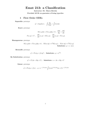
1 First Order ODEs
Separable: prototype
dy
y = h(y)f (x) ; = f (x)dx
h(y)
Exact: prototype
∂M ∂N
M (x, y)dx + N (x, y)dy = 0 ; =
∂y ∂x
∂F ∂F
F (x, y) = C , (x, y) = M (x, y) ; (x, y) = N (x, y)
∂x ∂y
Homogeneous: prototype
M (x, y)dx + N (x, y)dy = 0 ; M (tx, ty) = td M (x, y) ; N (tx, ty) = td N (x, y)
Substitute: y = x · u(x)
Bernoulli: prototype
1
y + P (x)y = f (x)y n ; Substitute: y = u 1−n
By Substitution: prototype
y = F (Ax + By + C) ; Substitute: u = Ax + By + C
Linear: prototype
y + P (x)y = f (x) ; y = e− P (x)dx
f (x)e P (x)dx
dx + Ce− P (x)dx
1

2. 2 Second (and higher) order Linear ODEs
Const-Coeffs (CC): prototype
ay + by + cy = f (x)
Auxiliary Eq. am2 + bm + c = 0

 c 1 e m1 x + c 2 e m2 x Real and distinct m1 , m2
yc = c1 e cos(βx) + c2 eαx sin(βx) Complex conjugate m1,2 = α ± iβ
αx

c1 emx + c2 x emx Only one root m1 = m2 = m
yp = By undetermined coefficients or Variation of parameters
Cauchy–Euler: prototype
a x2 y + b x y + c y = f (x) , (x > 0)
Auxiliary Eq. am(m − 1) + bm + c = 0

 c 1 x m1 + c 2 x m2 Real and distinct m1 , m2
yc = c1 x cos(β ln(x)) + c2 xα sin(β ln(x))
α
Complex conjugate m1,2 = α ± iβ

c1 xm + c2 ln(x) xm Only one root m1 = m2 = m
yp = Variation of parameters
Variation of Parms : put in normal form the equation
y + P (x)y + Q(x)y = f (x)
Find complementary solutions y1 and y2 then
yp = u 1 y1 + u 2 y2
−y2 f (x) y1 f (x)
u1 = ; u2 =
W W
y1 y2
W := det = y 1 y2 − y 1 y2
y1 y2
3 Series and solution by series (centered at x=0)
y + P (x)y + Q(x)y = 0
∞
y= cn x n = c 0 + c 1 x + c 2 x 2 + c 3 x 3 + c 4 x 4 + c 5 x 5 + . . .
n=0
4 Homogeneous Systems
• Being able to convert from system form to matrix form and viceversa.

 x1 = a11 x1 + · · · + a1n xn

.
.
 .

xn = an1 x1 + · · · + ann xn
   
a11 · · · a1n x1
. .  .
X = AX , A= . . .
. ; X= .  .
an1 · · · ann xn
2

3. • Find Eigenvalues and Eigenvectors of A
det(A − λI) = 0 ⇒ λ1 , . . . ,
A − λI K = λK
(a) Matrix is diagonalizable (n eigenvectors) and eigenvalues are real
X = c 1 e λ1 t K 1 + . . . + c n e λn t K n
(b) There are repeated eigenvalues and less than n eigenvectors; e.g. λ 1
has multiplicity 2 but there is only one eigenvector
X1 = c1 eλ1 t K + c2 eλ1 t (tK + P)
A − λ1 I P = K
(c) There are complex conjugate eigenvalues: find complex eigenvector
and split in real and imaginary part.
λ = α ± iβ
K = A ± iB
αt
X1 = e A cos(βt) − B sin(βt)
X2 = eαt A sin(βt) + B cos(βt)
• Solution by exponentiation
Φ(t) = eAt
5 Nonhomogeneous Systems
In matrix form
X = AX + F(t)
Complementary solution from above, particular solution by
1. Variation of parameters
Xp = Φ(t) Φ(t)−1 F(t) dt
2. Diagonalization
X = P Y ; Y = DY + P −1 F(t)
 
λ1 0 · · ·
 0 λ2 
D= .
 . .. 

. .
0 λn
3