Downloaded 642 times
![Univariate Analysis/Descriptive Statistics
• Variance
– One measure of dispersion (deviation from the mean) of a data
set. The larger the variance, the greater is the average deviation
of each datum from the average value.
=
−∑=
m
mm
N
N
i
i
2
1
)(
1
Variance =
Average value of the data set
Variance = [(45 – 68.6)2
+ (49 – 68.6)2
+ (50 – 68.6)2
+ (53 – 68.6)2
+ …]/20 = 181
Excel Functions: VARP(), VAR()
20](https://image.slidesharecdn.com/univariatebivariateanalysishypothesistestingchisquare-150526014604-lva1-app6891/75/Univariate-bivariate-analysis-hypothesis-testing-chi-square-20-2048.jpg)
![Univariate Analysis/Descriptive Statistics
• Standard Deviation
– Square root of the variance. Can be thought of as the
average deviation from the mean of a data set.
– The magnitude of the number is more in line with the
values in the data set.
Standard Deviation = ([(45 – 68.6)2
+ (49 – 68.6)2
+ (50 – 68.6)2
+ (53 – 68.6)2
+
…]/20)1/2
= 13.5
Excel Functions: STDEVP(), STDEV()
21](https://image.slidesharecdn.com/univariatebivariateanalysishypothesistestingchisquare-150526014604-lva1-app6891/75/Univariate-bivariate-analysis-hypothesis-testing-chi-square-21-2048.jpg)


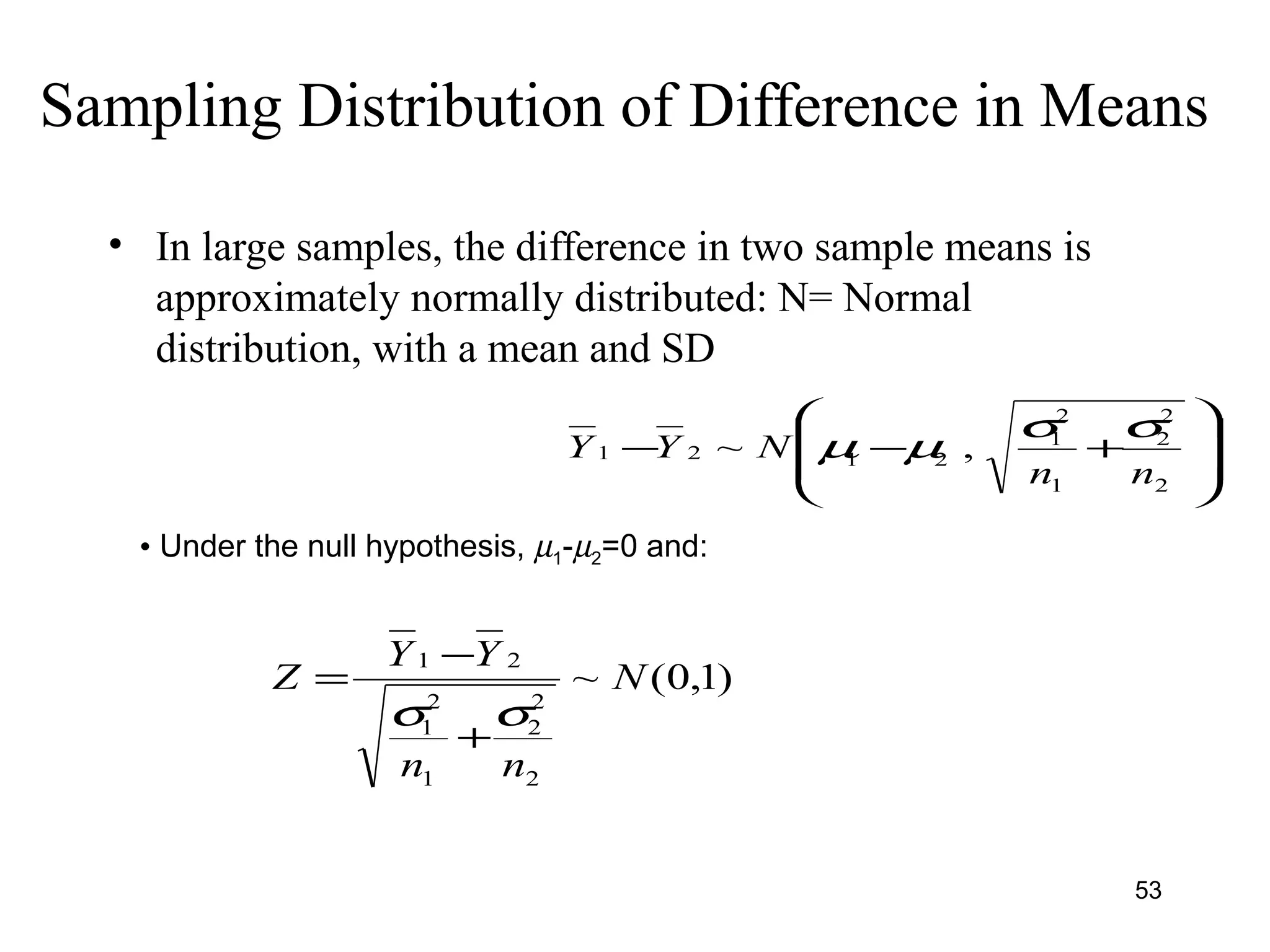
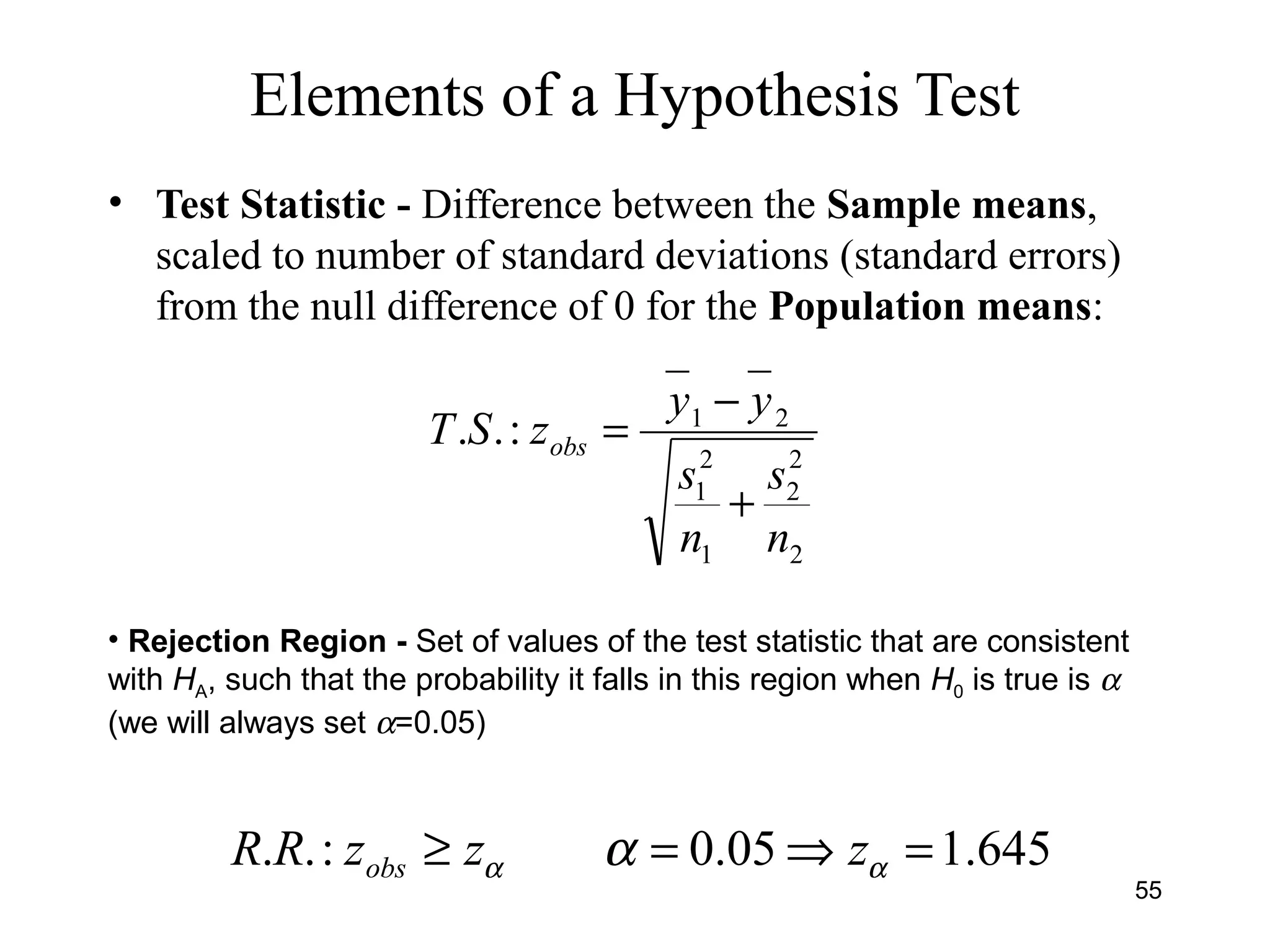
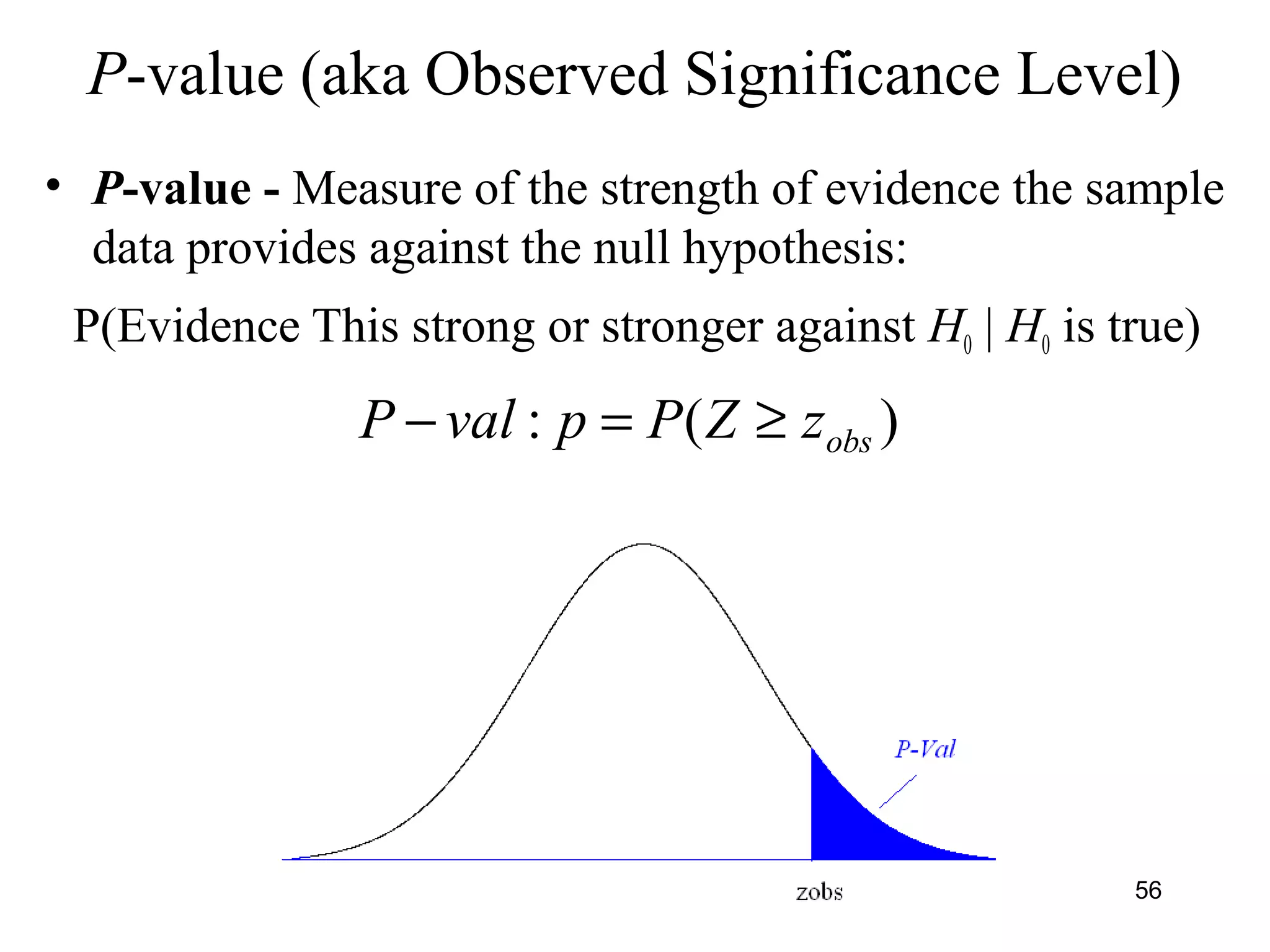
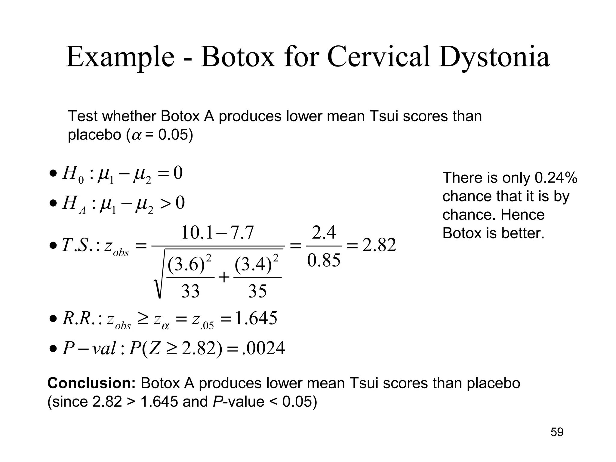
![Large-Sample Test H0:µ1-µ2=0 vs H0:µ1-µ2>0
• H0: µ1-µ2 = 0 (No difference in population means
• HA: µ1-µ2 > 0 (Population Mean 1 > Pop Mean 2)
ty_value][probabiliobs
obs
2
2
2
1
2
1
21
obs
)zZ(P:valueP
zz:.R.R
n
s
n
s
yy
z:.S.T
Region][Rejection
Statistic][Test
=≥−•
≥=•
+
−
==•
α
• Conclusion - Reject H0 if test statistic falls in rejection region, or
equivalently the P-value is ≤ α
57](https://image.slidesharecdn.com/univariatebivariateanalysishypothesistestingchisquare-150526014604-lva1-app6891/75/Univariate-bivariate-analysis-hypothesis-testing-chi-square-57-2048.jpg)


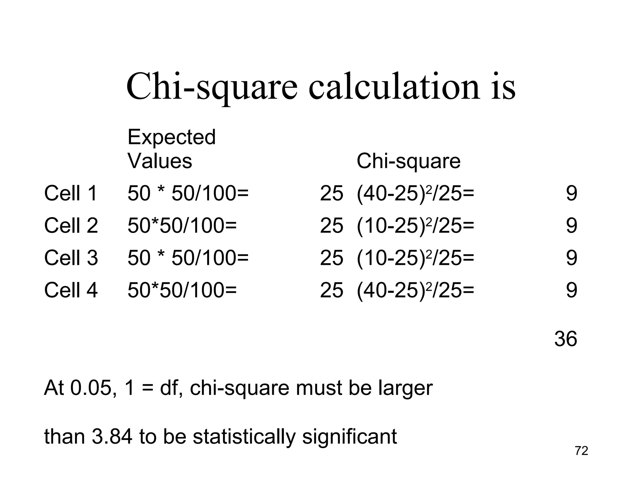
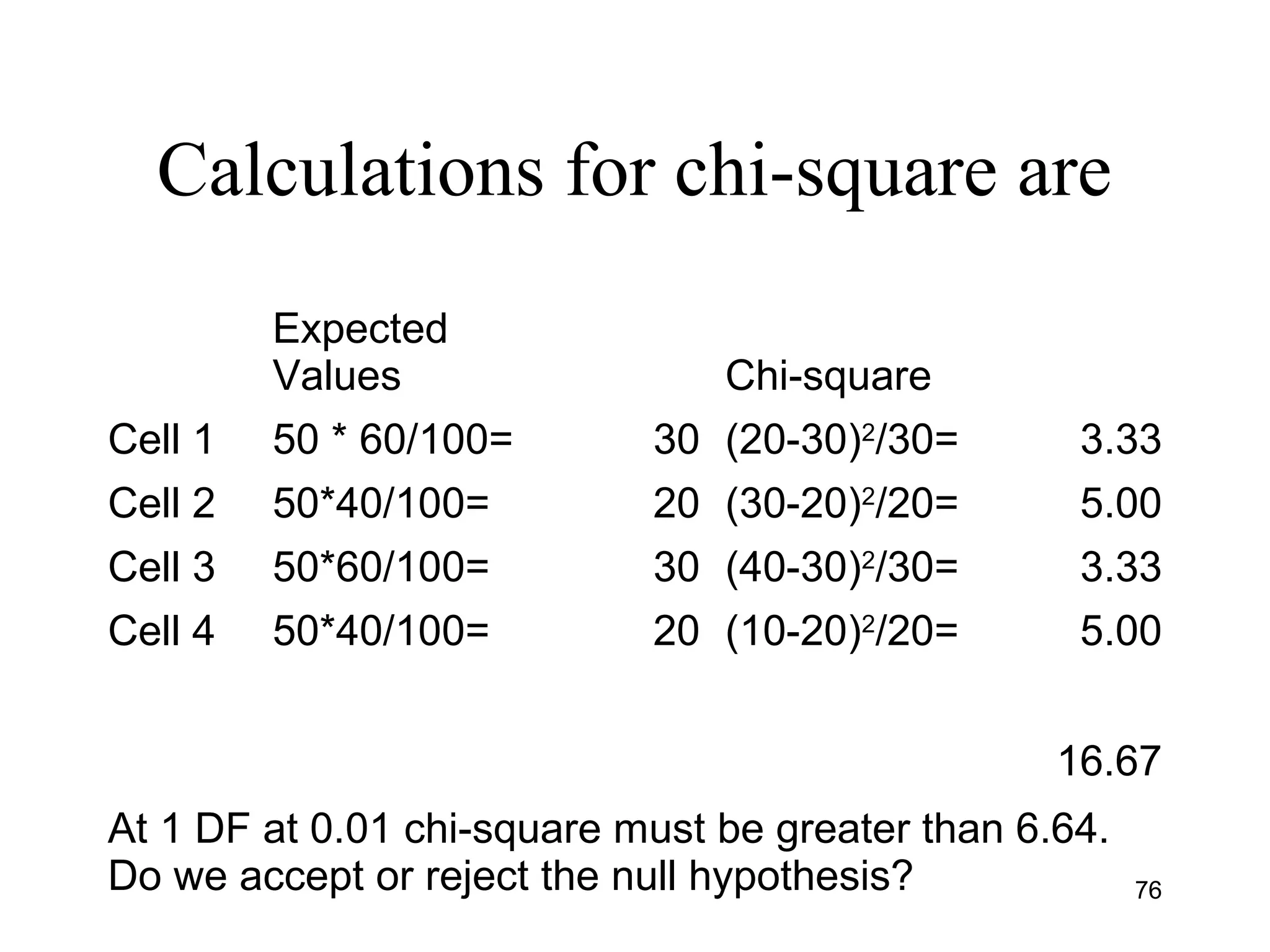
![Calculating Chi-Square
• Formula is [0 - E]2
E
Where 0 is the observed value in a cell
E is the expected value in the same
cell we would see if there was no
association
67](https://image.slidesharecdn.com/univariatebivariateanalysishypothesistestingchisquare-150526014604-lva1-app6891/75/Univariate-bivariate-analysis-hypothesis-testing-chi-square-67-2048.jpg)
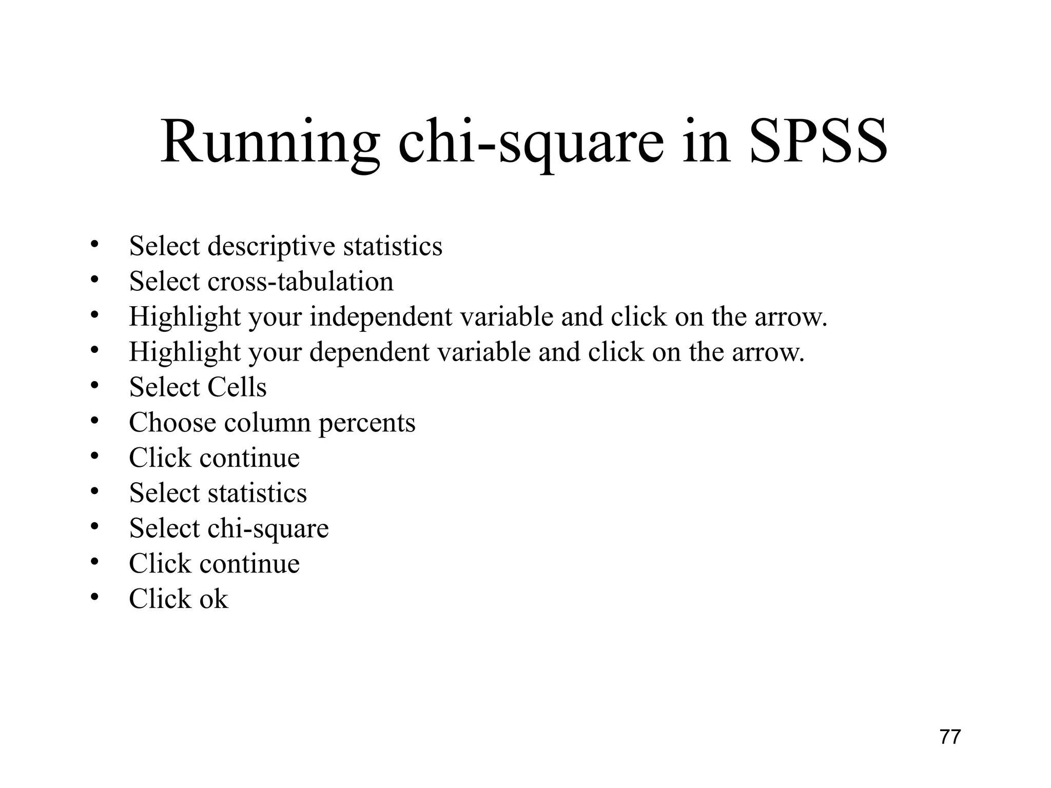

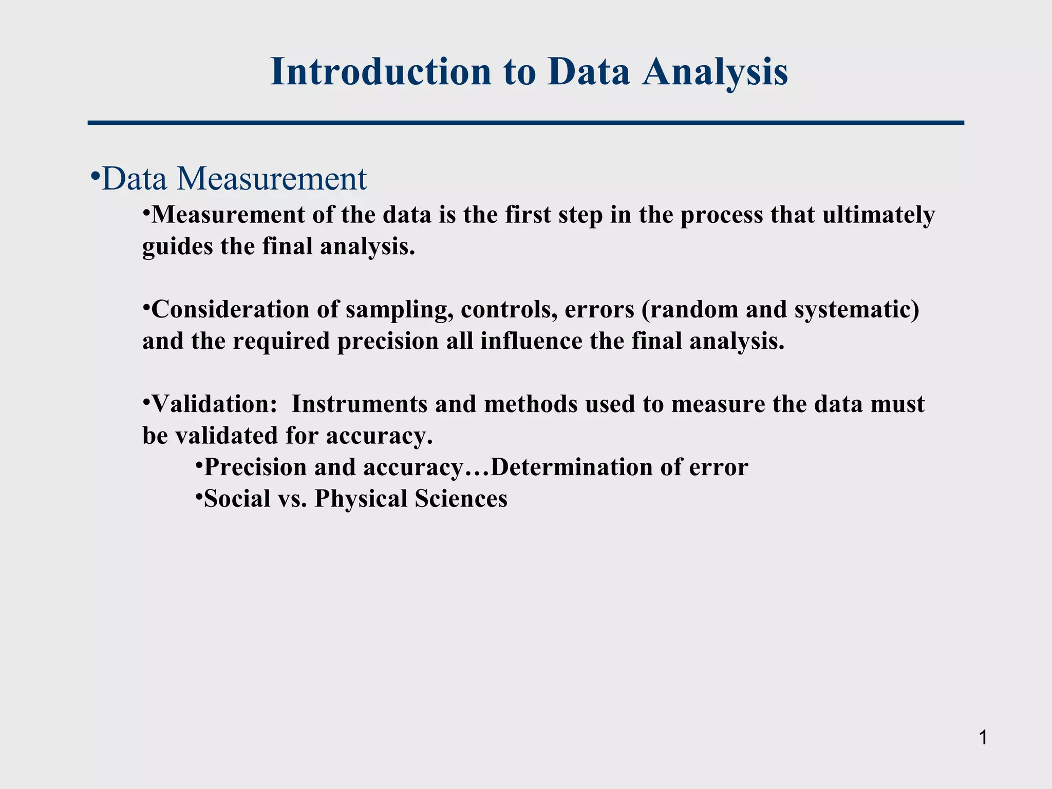
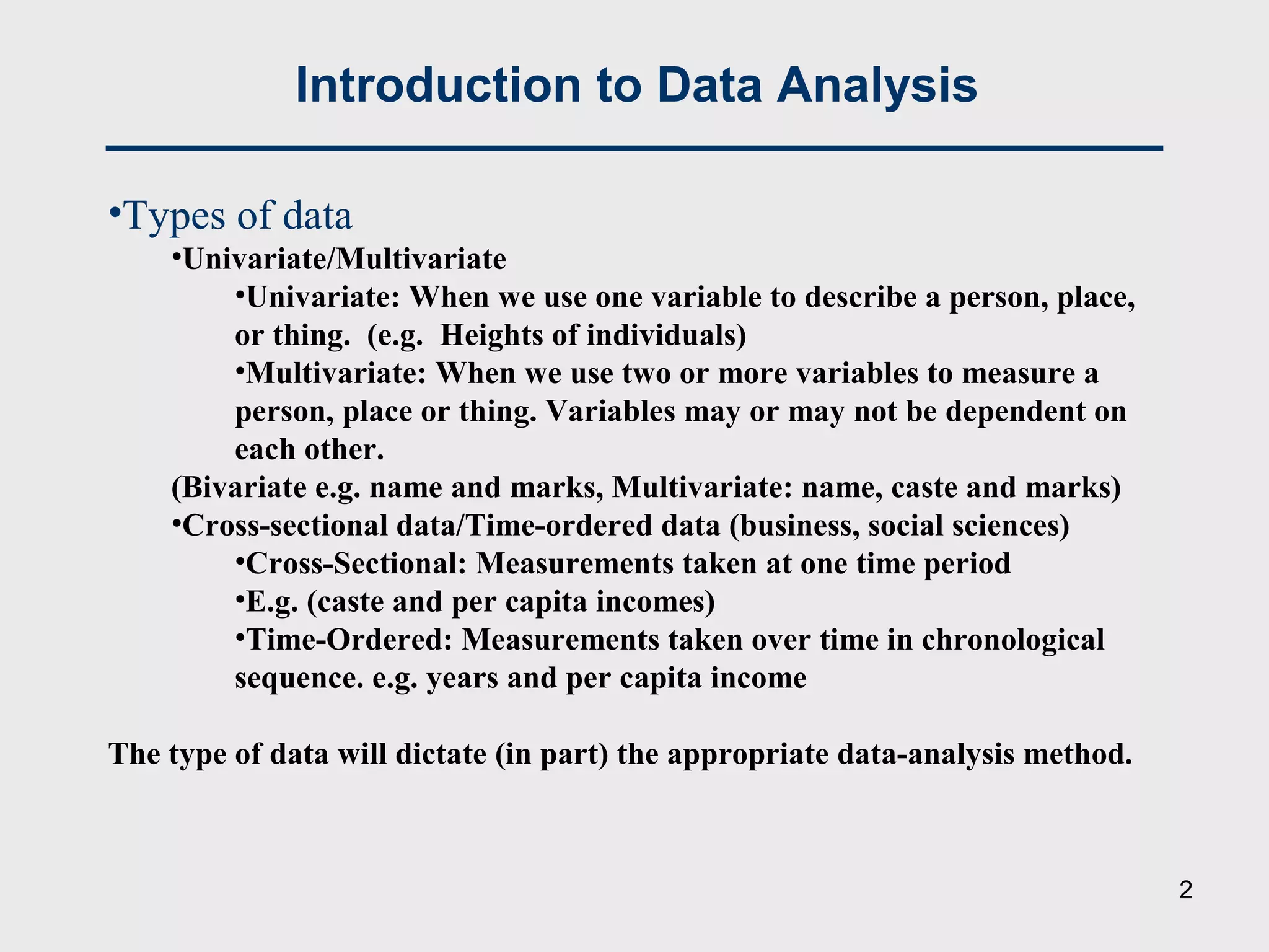
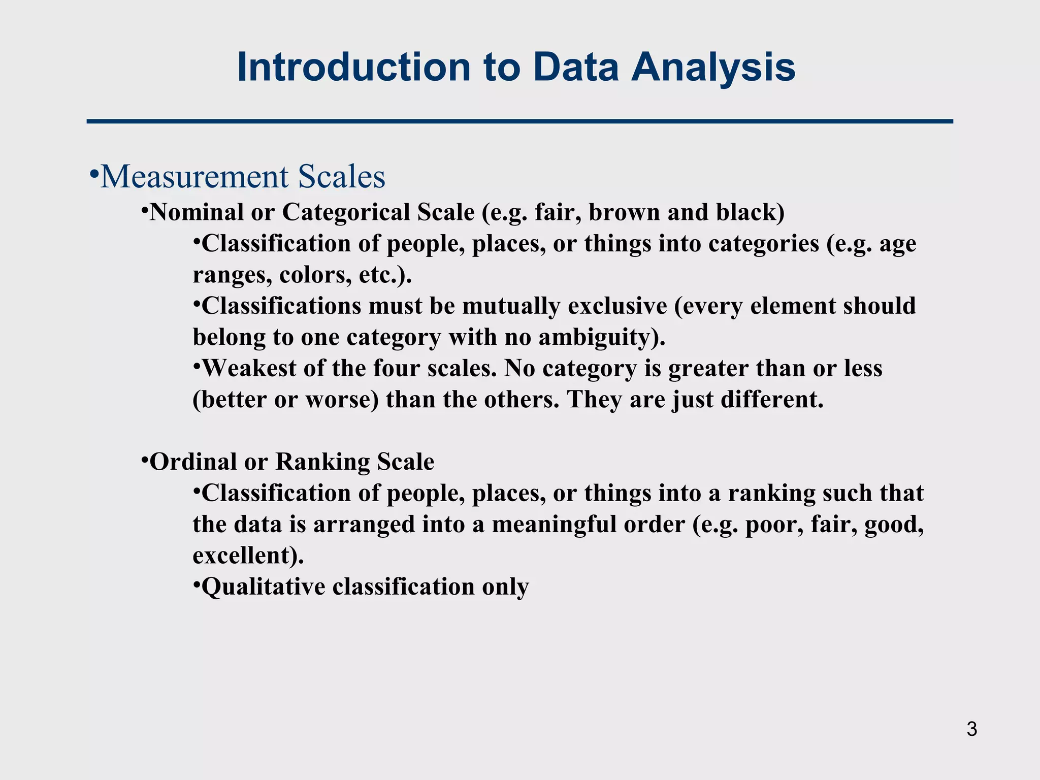
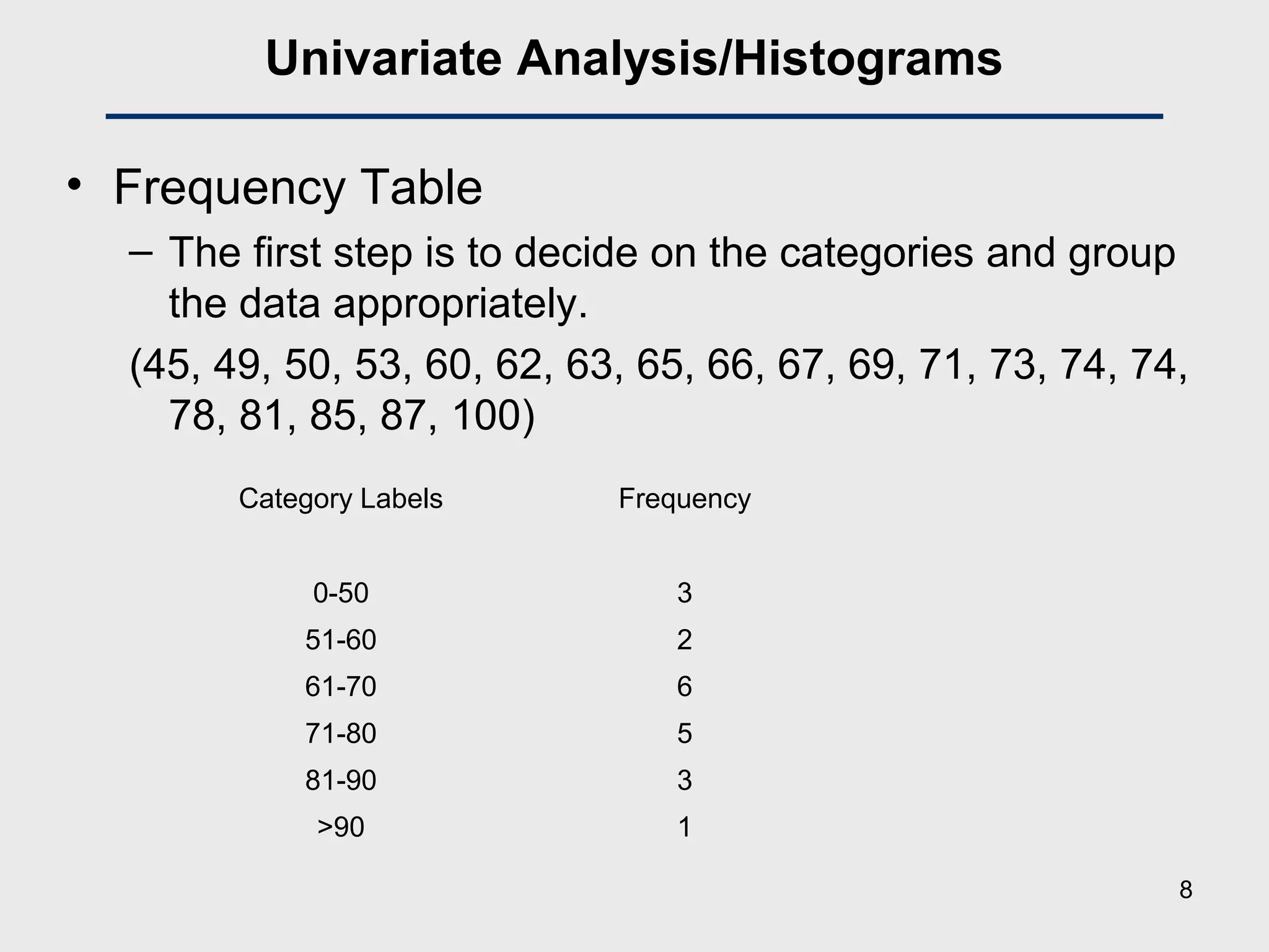
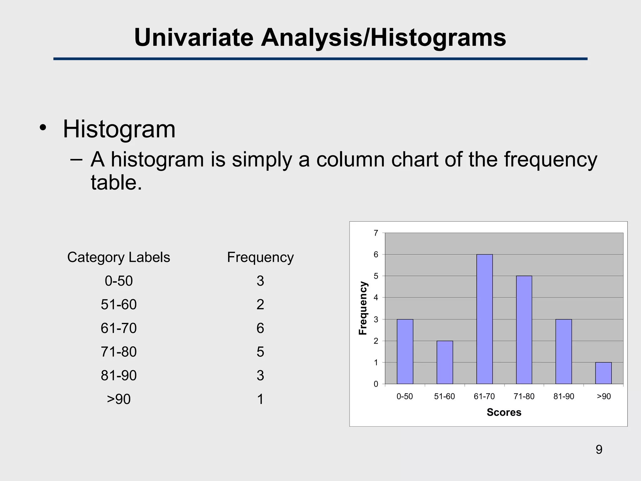
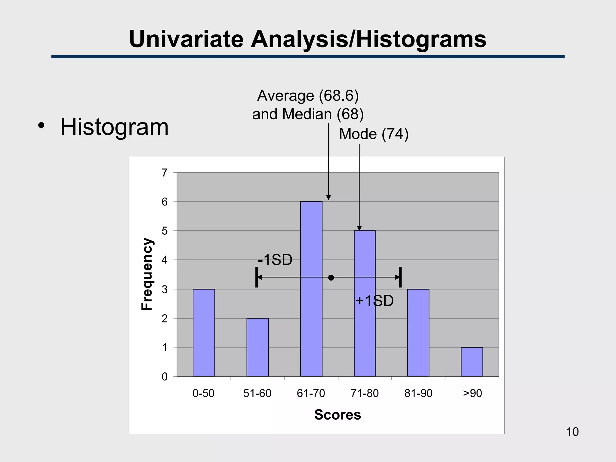
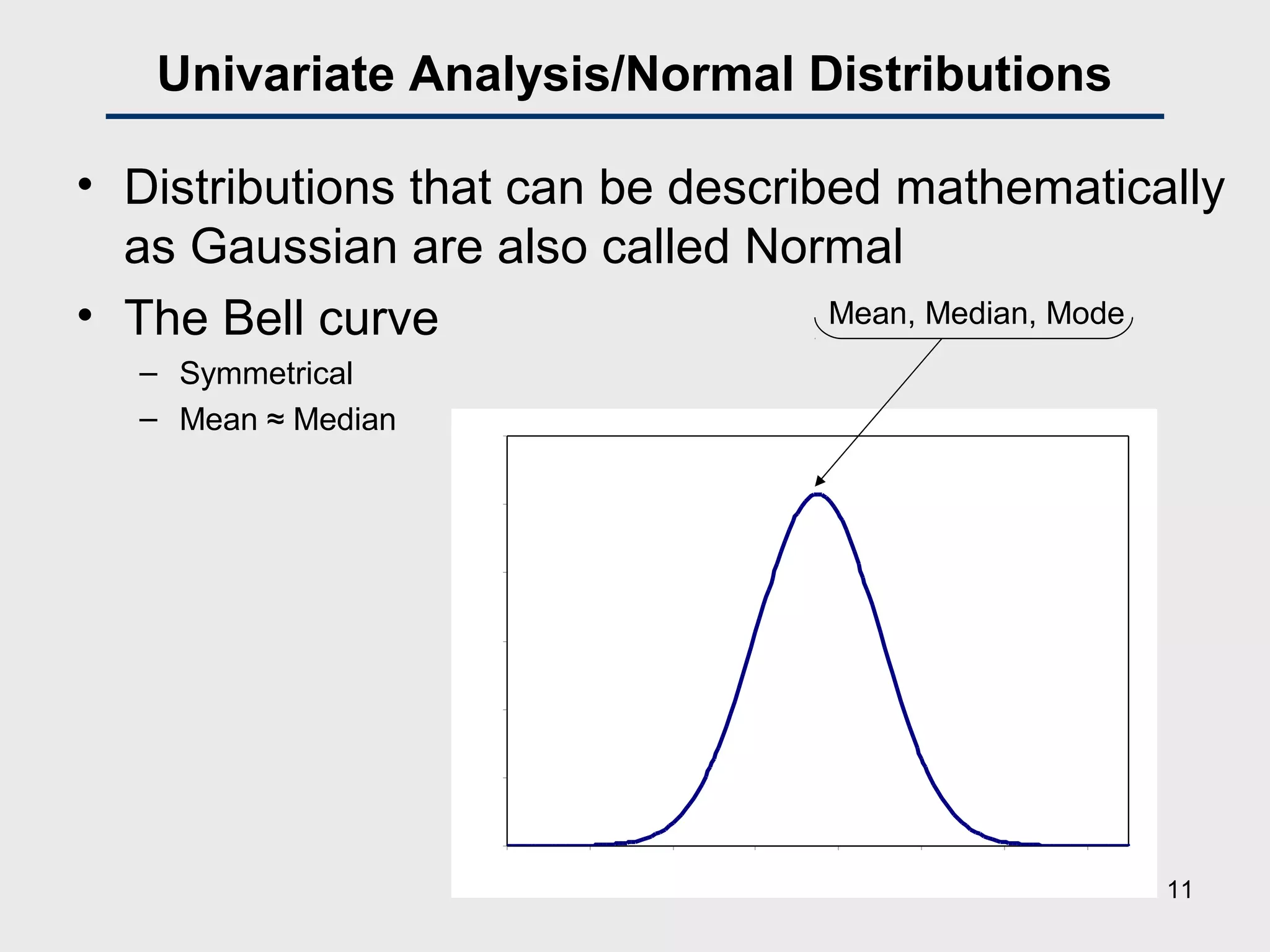
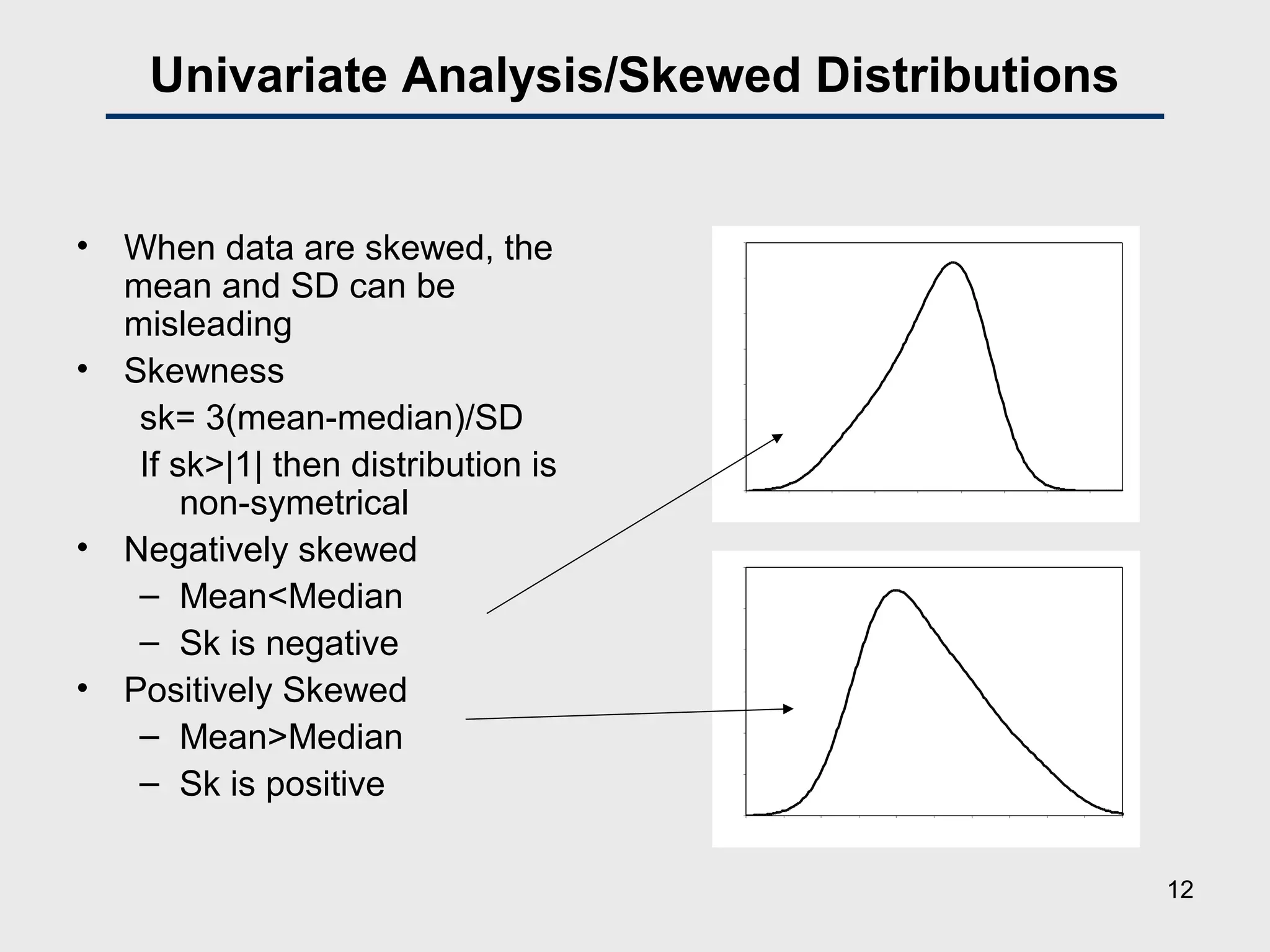
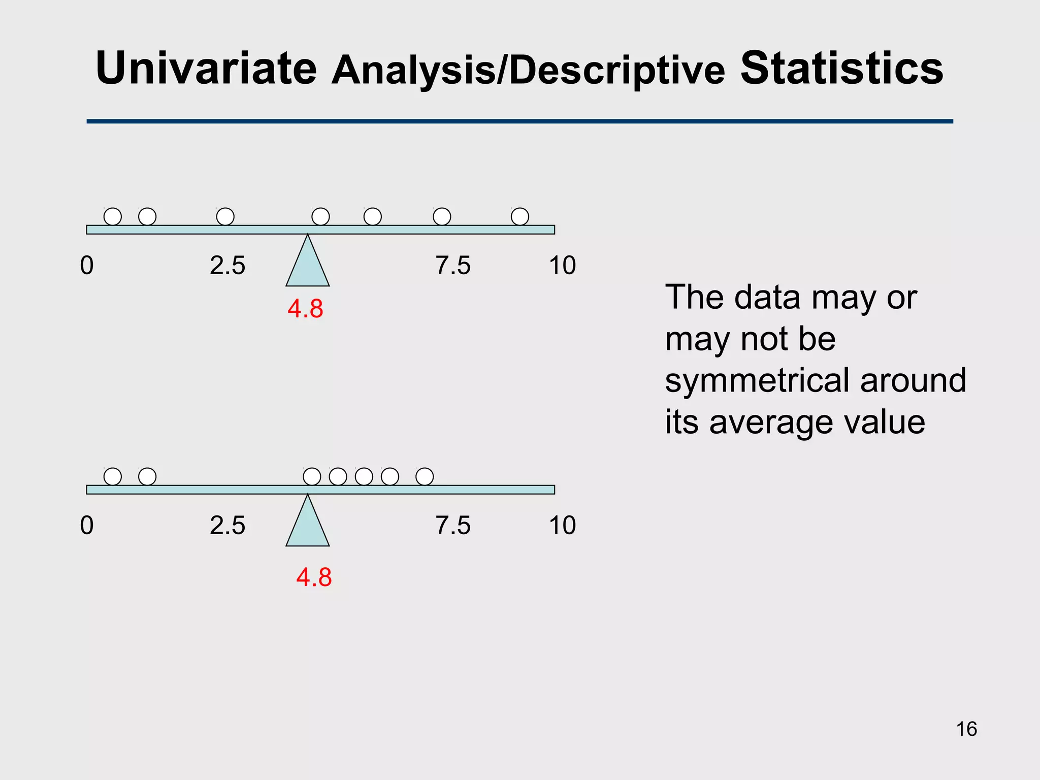
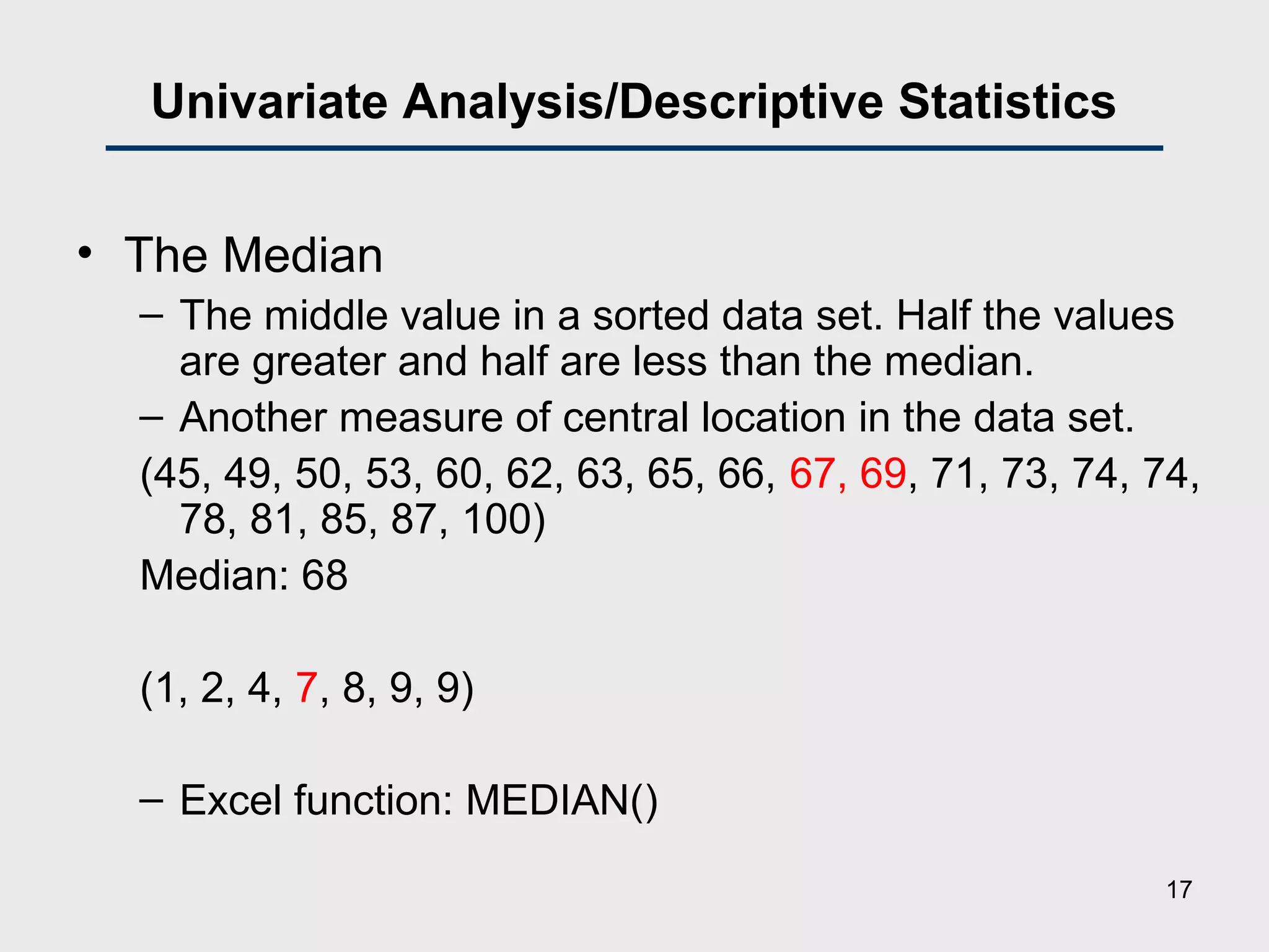
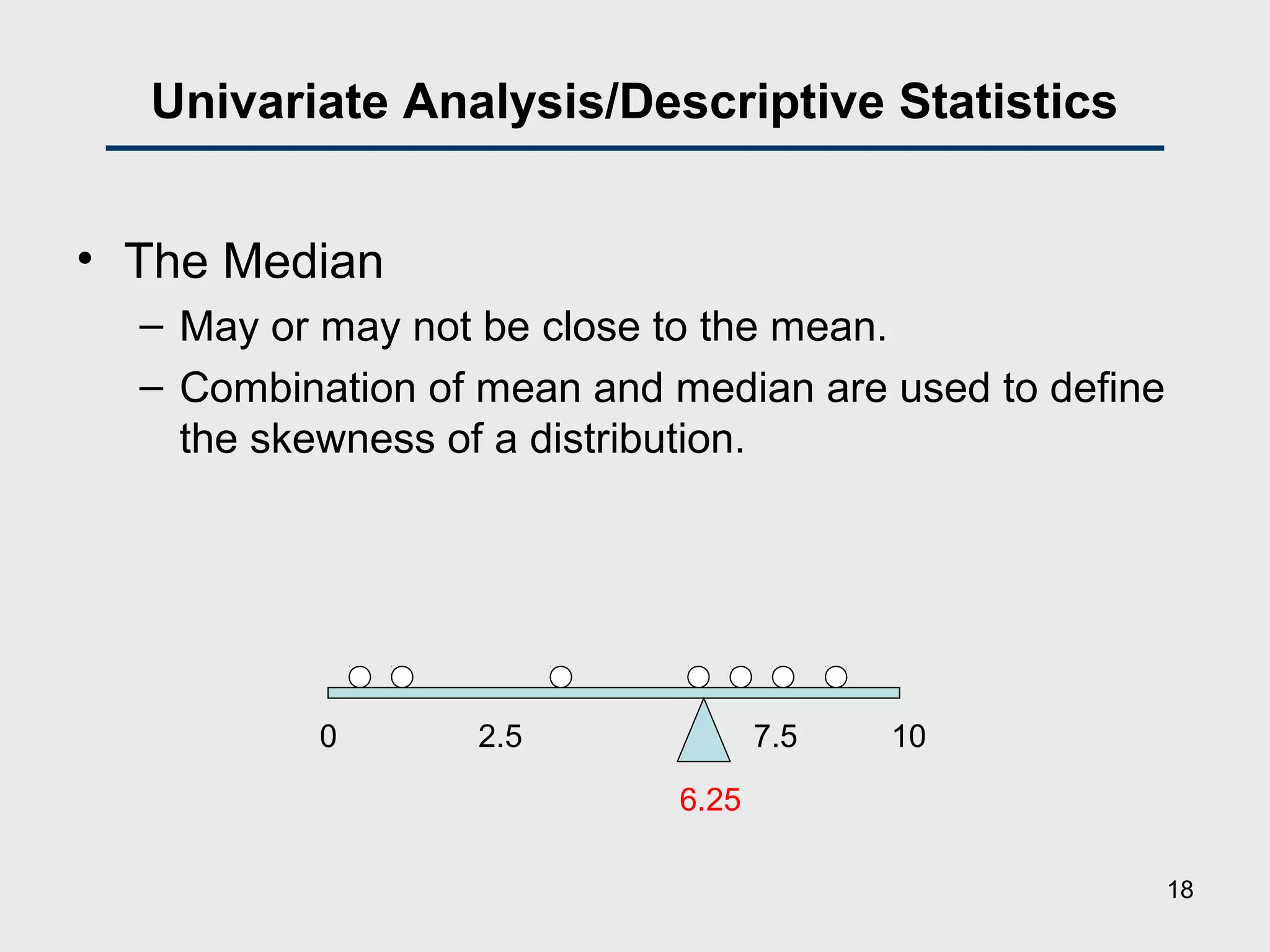
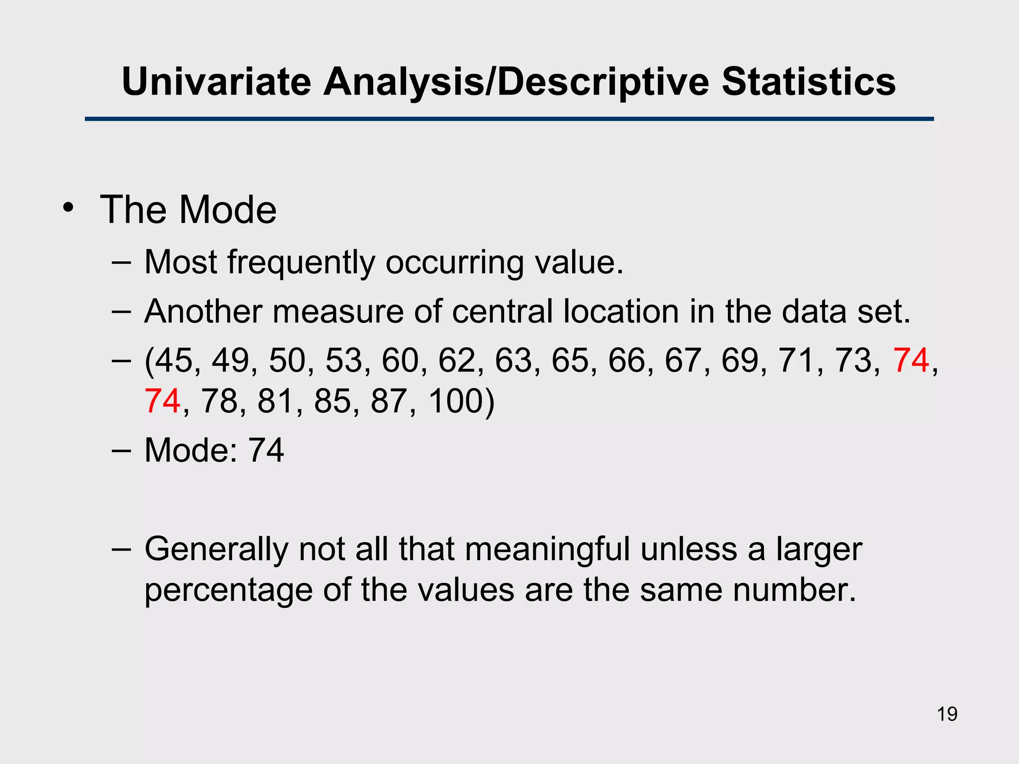
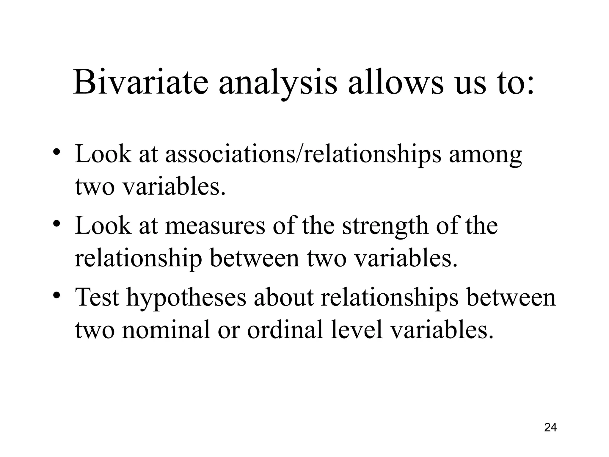
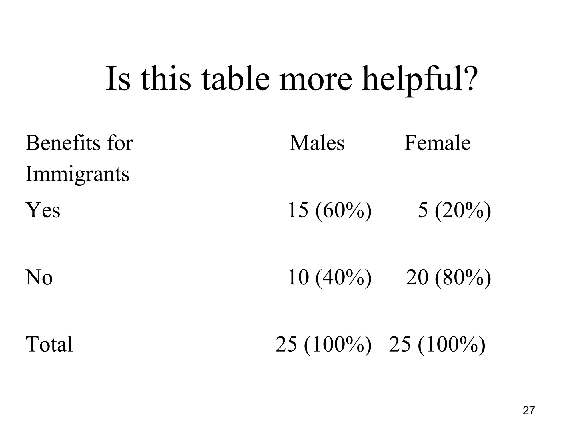
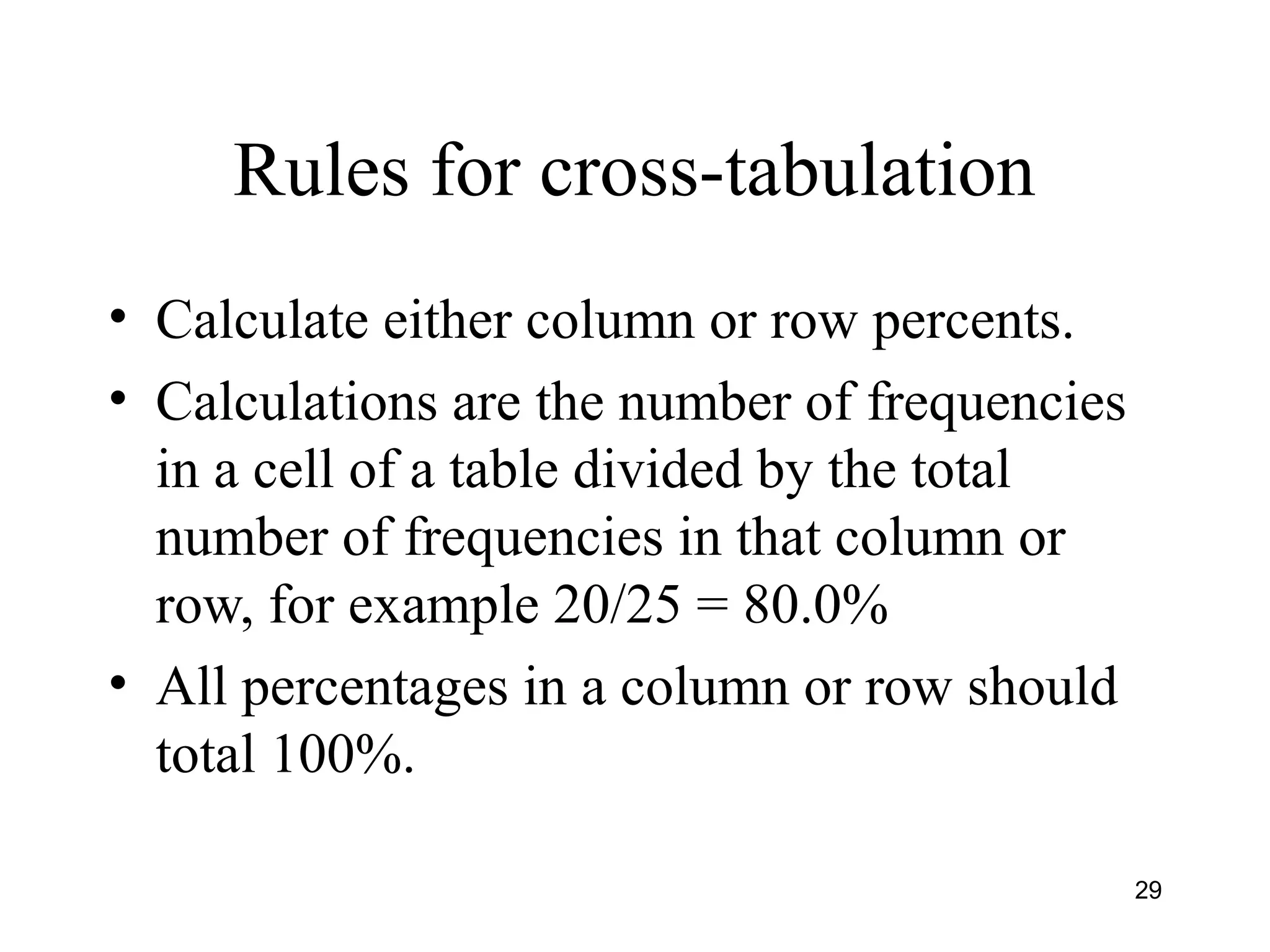
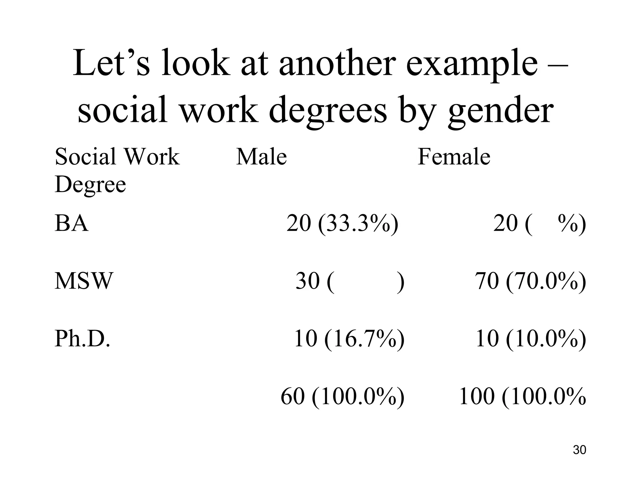
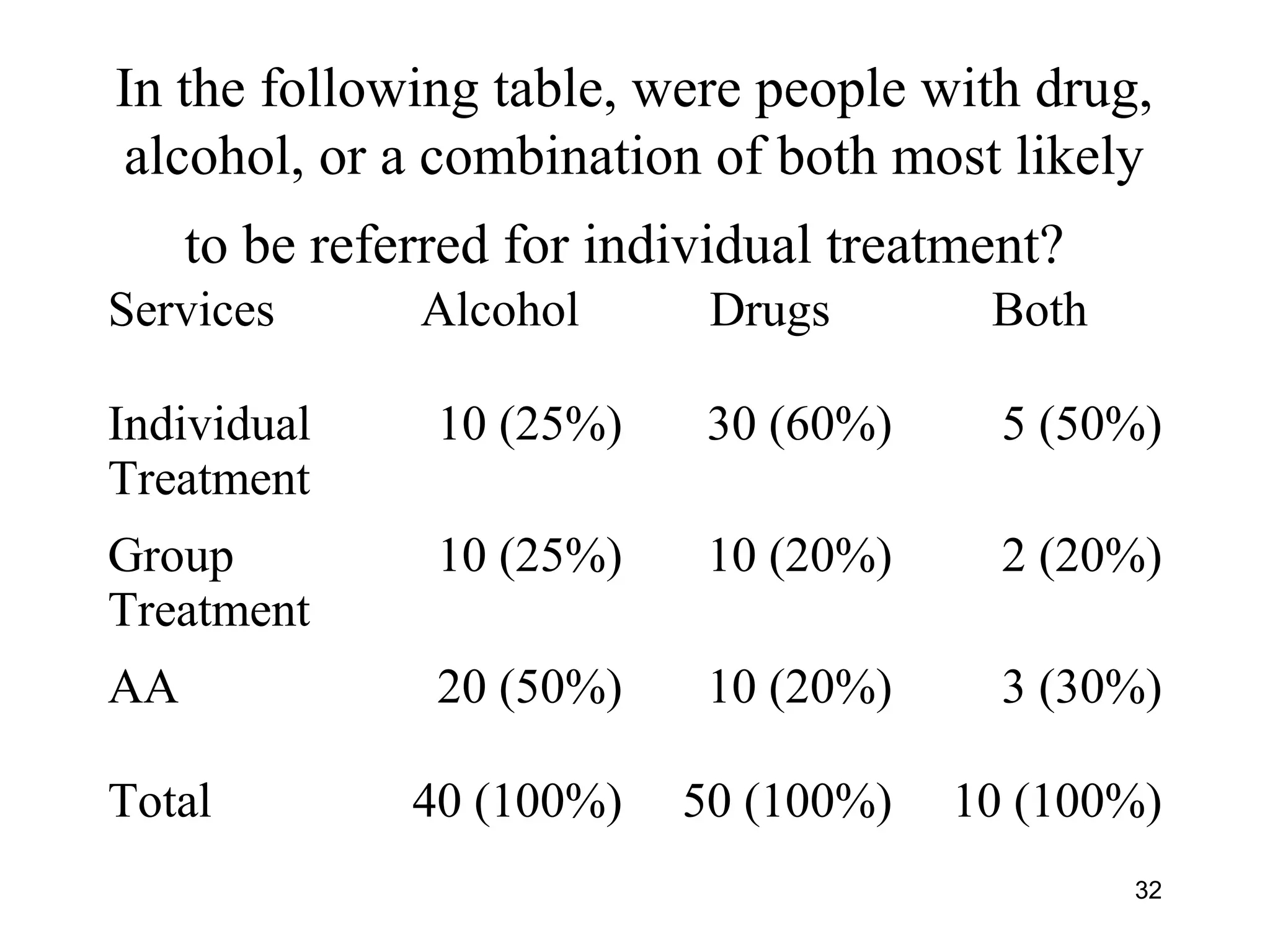
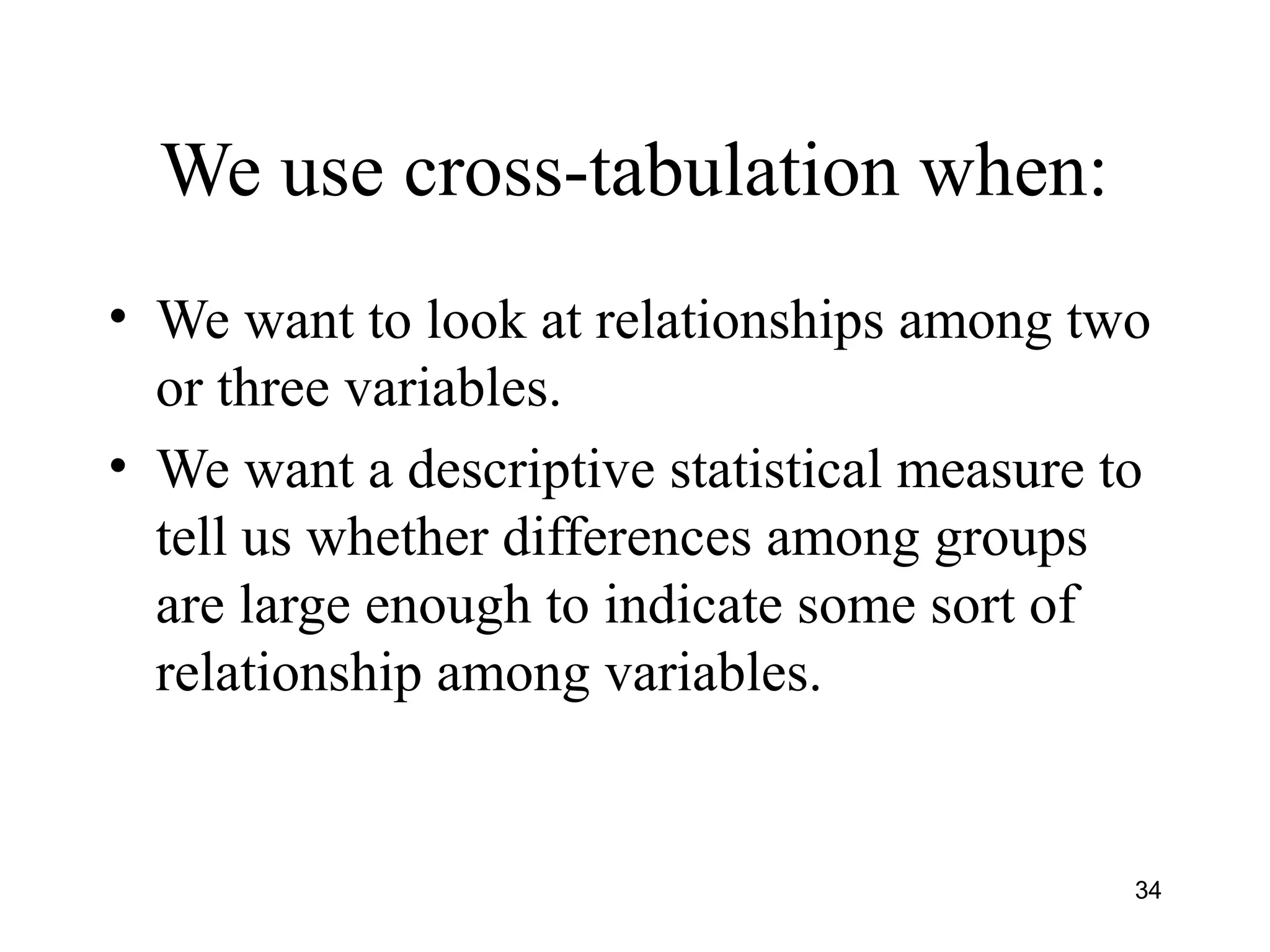
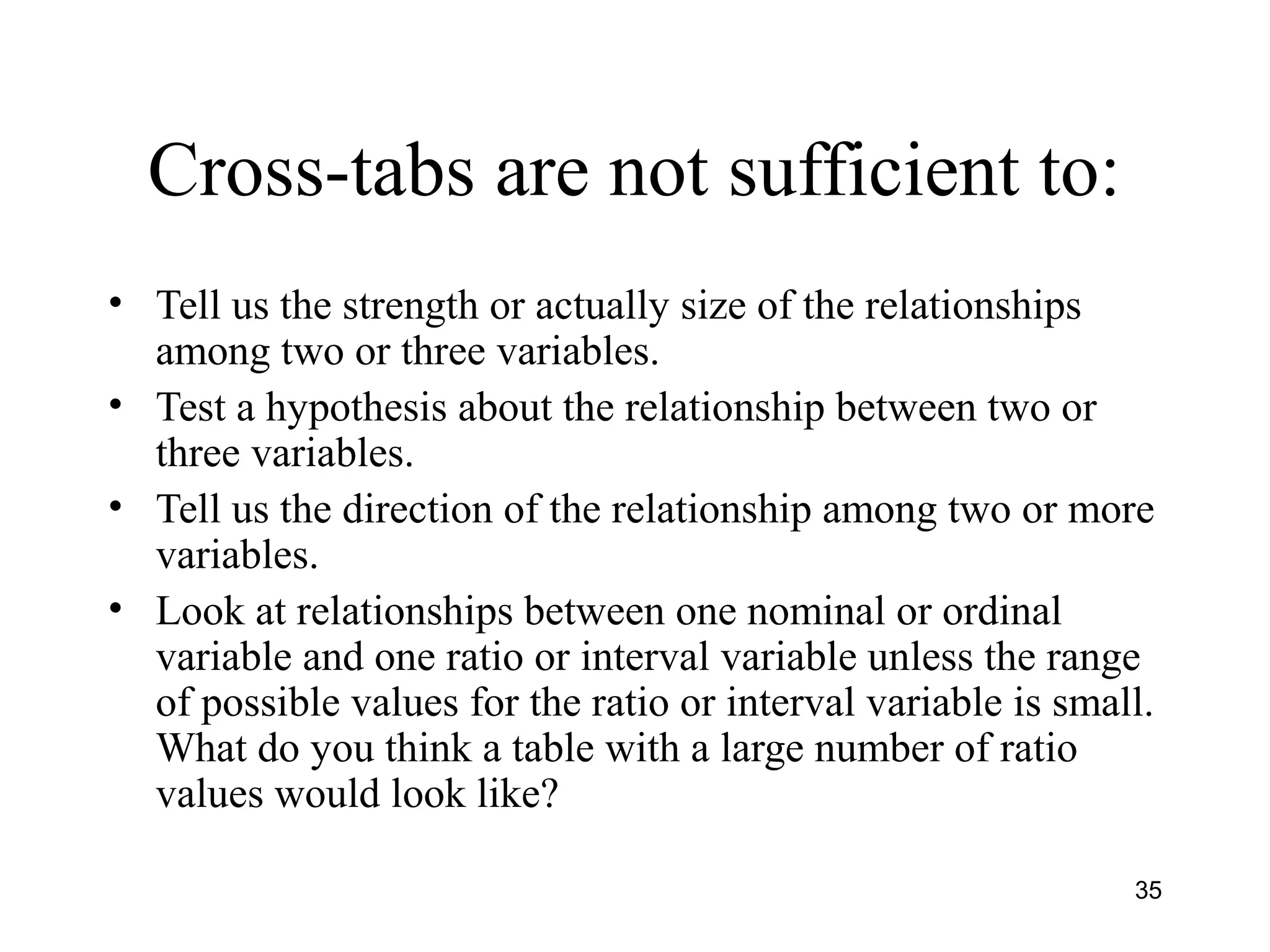
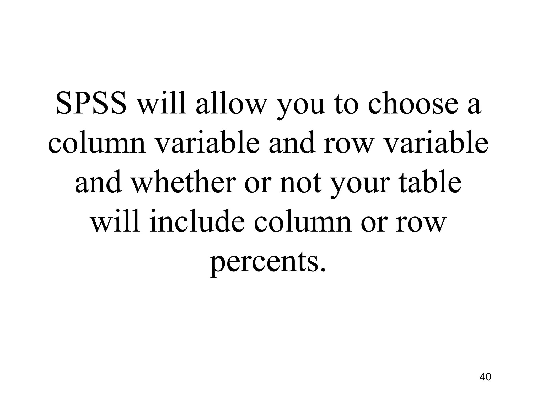
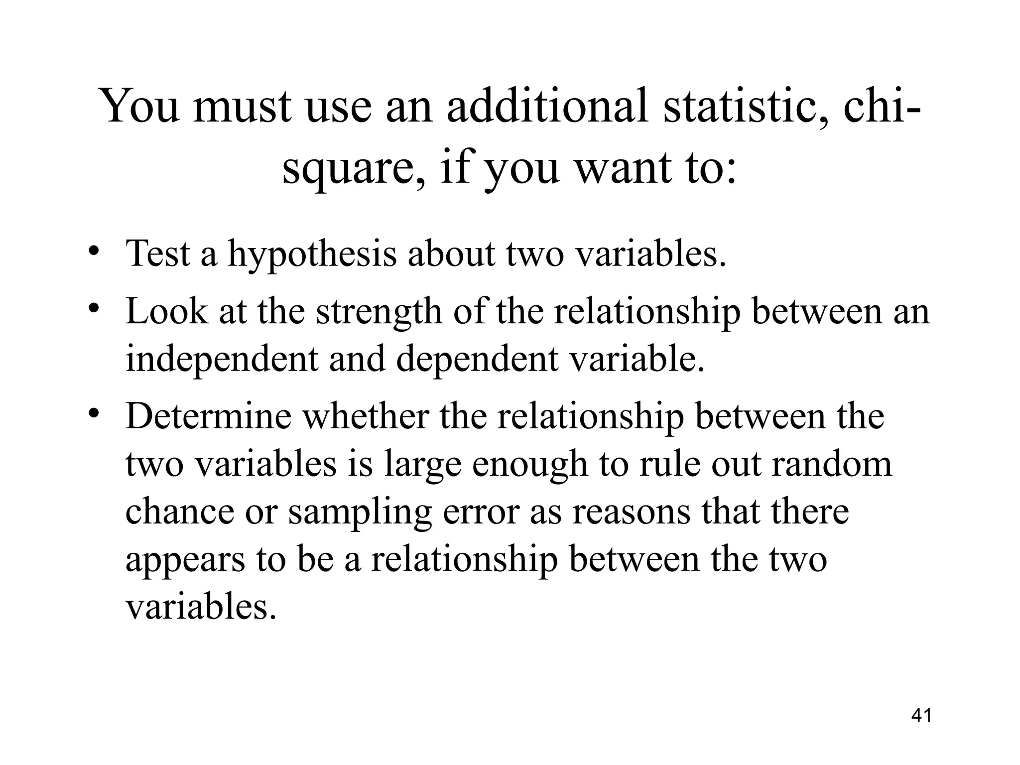
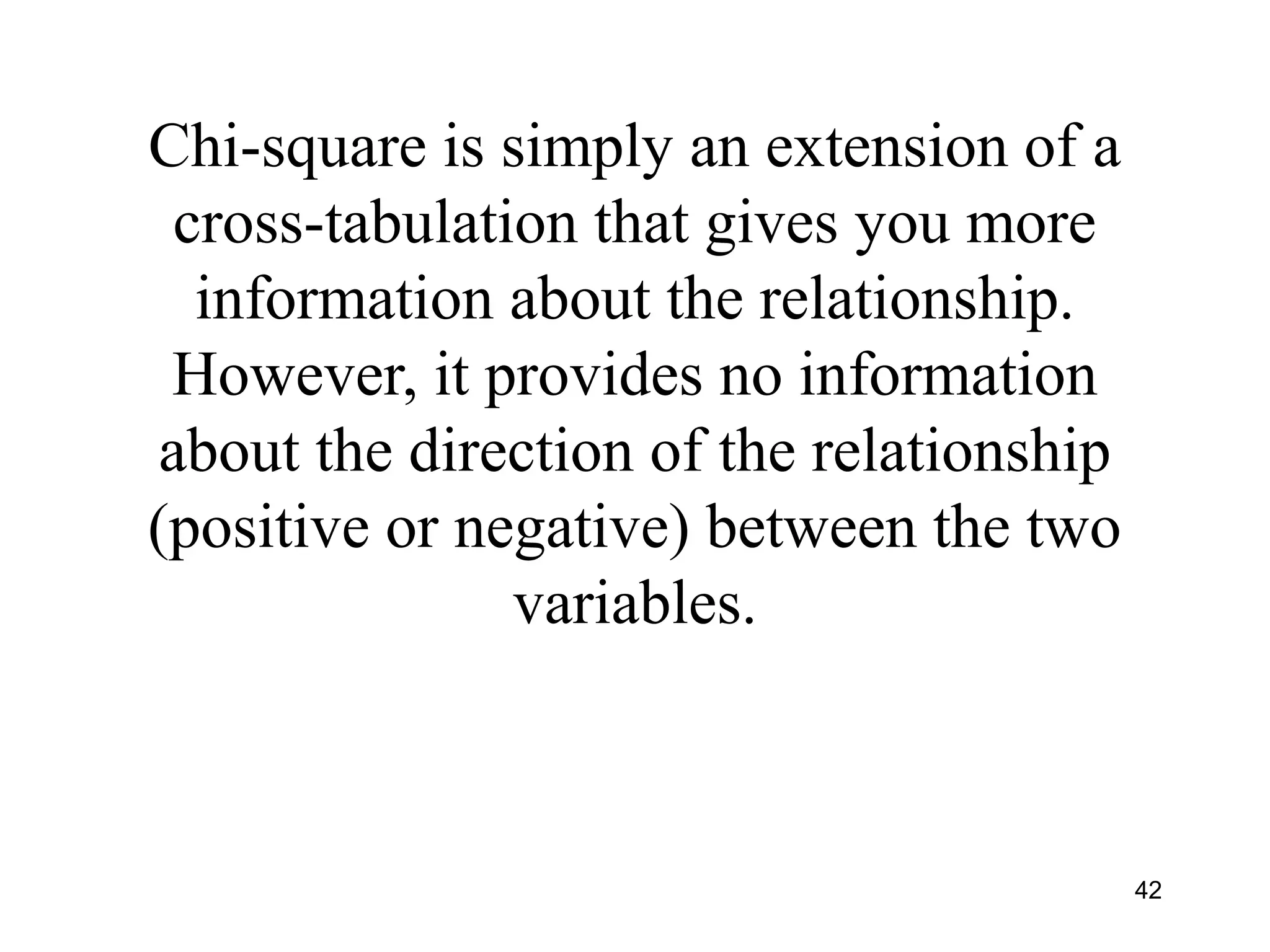
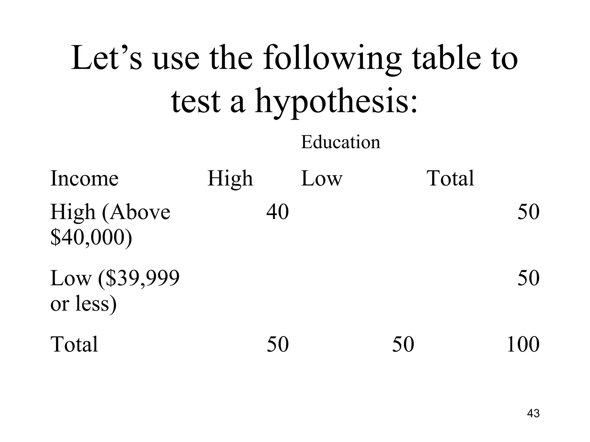
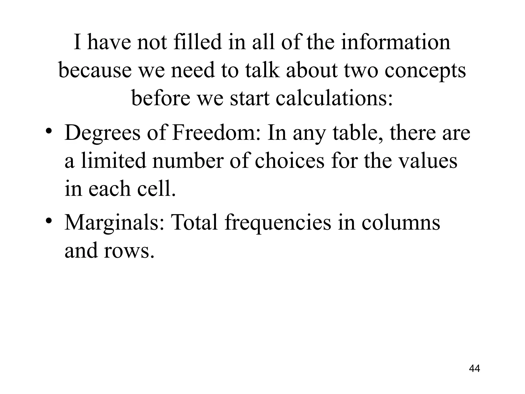
This document provides an introduction to data analysis. It discusses various topics related to measurement and types of data, including univariate and bivariate analysis. For univariate analysis, it describes descriptive statistics such as mean, median, mode, variance, and standard deviation. It also discusses data distributions and different measurement scales. For bivariate analysis, it introduces cross-tabulation and chi-square tests to examine relationships between two variables. Cross-tabulation allows looking at associations between variables through frequencies and percentages in tables, while chi-square can be used to test hypotheses about relationships and determine statistical significance.