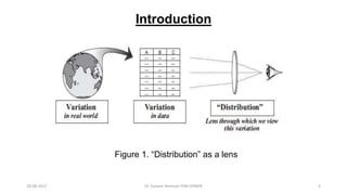
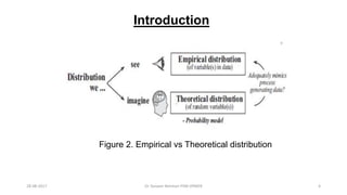
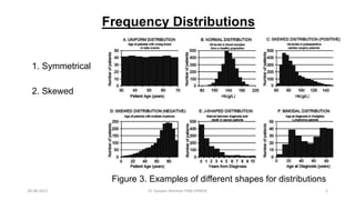
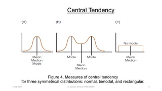
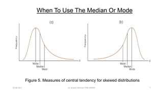
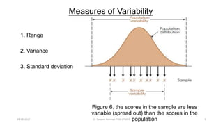
Statistical distributions

STATISTICAL
DISTRIBUTIONS
- Dr. TANVEER REHMAN
MODERATOR : Dr. VENKATACHALAM

OUTLINE
1. Introduction
2. Frequency distributions
3. Central tendency
4. Variability
5. Z score
6. Theoretical distributions
7. Application
28-08-2017 2Dr Tanveer Rehman PSM JIPMER

Figure 1. “Distribution” as a lens
Introduction

Figure 2. Empirical vs Theoretical distribution
Introduction

Figure 3. Examples of different shapes for distributions
Frequency Distributions
1. Symmetrical
2. Skewed

Figure 4. Measures of central tendency
for three symmetrical distributions: normal, bimodal, and rectangular.
Central Tendency

When To Use The Median Or Mode
Figure 5. Measures of central tendency for skewed distributions

Figure 6. the scores in the sample are less
variable (spread out) than the scores in the
population
Measures of Variability
1. Range
2. Variance
3. Standard deviation

Figure 7.Following a z-score transformation, the X-
axis is relabelled in z-score units.
Z or Standard Score
1. Purpose
2. Equation

Figure 8. The distribution of original score, a
z-score, and a new, standardized score.
Z-score Distributions
1. Mean
2. S.D.
3. Shape
4. Standardized distribution
5. Disadvantage

Distributions
Discrete
Symmetric
If clustered:
Binomial
Uniform
Discrete
Asymmetric Outliers
Mostly Positive:
Negative Binomial,
Poisson
Only Positive:
Geometric
Mostly Negative:
Hypergeometric
Continuous

Distributions
Discrete
Continuous
Symmetric
Not Clustered:
Uniform/
Multimodal
Outliers
No:
Triangular
Very Low:
Normal, t
Low:
Logistic, Cauchy
Asymmetric
Outliers Only Positive:
Exponential
Mostly Positive:
Chi-square, f, Lognormal, Gamma,
Weibull
Mostly Negative: Extreme28-08-2017 13Dr Tanveer Rehman PSM JIPMER

Figure 9. The normal distribution following a
z-score transformation.
Normal Distribution
1. Discoverer
2. Shape
3. Equation
4. Proportions

Figure 10. A portion of the unit normal table.

Application Of Normal Distribution
Q1. The population distribution of health expenditures is normal
with a mean of Rs. 5000 and a standard deviation of Rs. 1000.
What is the probability of randomly selecting an individual from
this population whose health expenditures is greater than Rs.
7000?

Key to Q1

First, the probability question is translated into a proportion
question: Out of all possible scores, what proportion is greater
than 700?
The mean is μ 500, so the score X 700 is to the right of the
mean. Because we are interested in all scores greater than 700,
we shade in the area to the right of 700. This area represents the
proportion we are trying to determine. Identify the exact position
of X > 700 by computing a z-score. For this example, That is, a
score of X 700 is exactly 2 standard deviations above the mean
and corresponds to a z-score of z2.00.. The proportion we are
trying to determine may now be expressed in terms of its z-
score:p(z > 2.00) ? all normal distributions regardless of the
values for μ and , have 2.28% of the scores in the tail beyond
z>2.00. Thus, for the population of scores, p(X >700) p(z=2.00)
2.28%

Figure 11 depicts the typical distribution of
sample means
Central Limit Theorem
1. Marquis de Laplace
2. The distribution of sample means
3. Any of two conditions to satisfy

Figure 12 shows that the size of the
standard error decreases as the
sample size increases.
Standard Error of M
1. Serves the same two purposes
2. The overall mean is equal to μ
3. SD is the “starting point”

Q2. A positively skewed distribution has μ = 60 and σ = 8.
a. What is the probability of obtaining a sample mean greater than M = 62
for a sample of n = 4 scores?
b. What is the probability of obtaining a sample mean greater than M = 62
for a sample of n = 64 scores?

Key to Q2.
a. The distribution of sample means does not satisfy either of the
criteria for being normal.
Therefore, you cannot use the unit normal table, and it is impossible to
find the probability.
b. With n = 64, the distribution of sample means is nearly normal. The
standard error is
8/ square root 64 = 1, the z-score is = 2.00, and the probability is
0.0228

Figure 13. The critical region (very unlikely
outcomes) for α = 0.05.
Hypothesis testing
1. State the hypothesis
2. Set the criteria for a decision
3. Collect data and compute
sample statistics
4. Make a decision

Q3. A health care project begins with a known population of all PHC staff—in this
case, scores on a standardized test that are normally distributed with µ = 65 and
σ = 15.
The Project officer suspects that special training in reading skills will produce a
change in the scores for the staff. Because it is not feasible to administer the
treatment (the special training) to everyone in the population, a sample of n = 25
individuals is selected, and the treatment is given to this sample.
Following treatment, the average score for this sample is M = 70. Is there
evidence that the training has an effect on test scores?

Key to Q3
State the hypothesis and select an alpha level. The null hypothesis states that
the special training has no effect. In symbols, H0: µ=65 (After special training,
the mean is still 65.) The alternative hypothesis states that the treatment
does have an effect. H1: µ is not equal to 65 (After training, the mean is
different from 65.) At this time you also select the alpha level. For this
demonstration, we will use α=0.05. Thus, there is a 5% risk of committing a
Type I error if we reject H0. Locate the critical region. With alpha .05, the
critical region consists of sample means that correspond to z-scores beyond
the critical boundaries of z=1.96. Obtain the sample data, and compute the
test statistic. For this example, the distribution of sample means, according
to the null hypothesis, is normal with an expected value of mean 65 and a
standard error of 3. In this distribution, our sample mean of M=70
corresponds to a z-score of 1.67 Make a decision about H0, and state the
conclusion. The z-score we obtained is not in the critical region. This
indicates that our sample mean of M=70 is not an extreme or unusual value
to be obtained from a population with mean = 65. Therefore, our statistical
decision is to fail to reject H0. Our conclusion for the study is that the data
do not provide sufficient evidence that the special training changes test
scores.

Figure 14 shows t distributions have more variability,
indicated by the flatter and more spread-out shape.
t Distribution
1. W. S. Gossett
2. Use
3. t statistic formula
4. Every sample like z-score
5. Approximation depends on df
6. Shape

Application Of t Distribution
Q4. A research project by Central Government would like to determine
whether there is a relationship between depression and aging.
It is known that the general population averages μ = 40 on a standardized
depression test.
The project officer obtains a sample of n = 9 individuals who are all more
than 70 years old.
The depression scores for this sample are as follows: 37, 50, 43, 41, 39, 45,
49, 44, 48.
On the basis of this sample, is depression for elderly people significantly
different from depression in the general population?

Key to Q4

H0: μ = 40. With df = 8 the critical values are t = +-2.306. For these
data, M = 44, SS = 162, s2 = 20.25, the standard error is 1.50, and t =
2.67.
Reject H0 and conclude that depression for the elderly is significantly
different from depression for the general population.

Figure 15 The binomial distribution is always a discrete
histogram, and the normal distribution is a continuous,
smooth curve
Binomial distributions
1. Two categories
2. Criteria for normality
3. Mean and SD
4. Z score

Application Of Binomial Distribution
Q5. A national health organization predicts that 50% of residents of a
particular area will get the flu this season. If a sample of 40 residents is
selected from the population, what is the probability that at least 26 of the
people will be diagnosed with the flu?

Key to Q5

Probability of flu = 0.50=p
q= 1- p= 0.5; n= 40
pn= 20 & qn=20, both above 10; so it’s a binomial distribution
Mean = pn = 20; SD= square root of npq= square root of 10 = 3.16
We are looking for 26 or more to get flu; so in a continuous data – real
lower limit is 25.5
Z score is 25.5-20 divided by 3.16= 1.74
In unit normal table, it comes to 4.09%

Figure 16 Chi-square distributions are
positively skewed. The critical region is placed
in the extreme tail, which reflects large chi-
square values.
Chi-square Distribution
1. Formula
2. Chi-square value
3. Characteristics

Application of Chi-square Distribution
Q6. Consider the following results from an influenza vaccine trial carried out
during an epidemic. Of 460 adults who took part, 240 received influenza
vaccination and 220 placebo vaccination. Overall 100 people contracted
influenza, of whom 20 were in the vaccine group and 80 in the placebo
group. We now wish to assess the strength of the evidence that vaccination
affected the probability of contracting influenza.

Key to Q6

Poisson Distribution
1. The number of discrete occurrences of an event during a period of time
2. Independent and random
3. The occurrences in each interval can range from zero to infinity
4. Depends upon just one parameter: the mean number of occurrences in
periods of the same length
28-08-2017 39
P(x) =
e -µµx
x!
Dr Tanveer Rehman PSM JIPMER

Figure 17. The distribution is very skewed for small means, when there is a
sizeable probability that zero events will be observed. It is symmetrical for large
means and is adequately approximated by the normal distribution for values of
λ=10 or more.

Application of Poisson distribution
Q7. A district health authority which plans to close the smaller of two
maternity units is assessing the extra demand this will place on the
remaining unit.
At present the larger unit averages 4.2 admissions per day and can cope
with a maximum of 10 admissions per day. This results in the unit’s capacity
being exceeded only on about one day per year.
After the closure of the smaller unit the average number of admissions is
expected to increase to 6.1 per day.
Estimate the proportion of days on which the unit’s capacity is then likely to
be exceeded.

Key to Q7

Figure 18 shows of all the values in the
distribution, only 5% are larger than F= 3.88,
and only 1% are larger than F =6.93.
F - Distribution
1. ANOVA
2. Advantage over t tests
3. F-ratio
4. Characteristics
5. Exact shape depends on df

Table 1. A portion of the F distribution table.

Application of F-distribution
Q8. A researcher obtains
F = 4.18 with df = 2,15.
Is this value sufficient to
reject H0 with α = 0.05?
Is it big enough to reject H0
if α = 0.01?

Thank You
There is an old saying that goes, “If it looks like a duck, walks like
a duck and quacks like a duck, then it is a duck.” If it
looks/walks/quacks like a duck, the statistician will use the
inferential reasoning appropriate for ducks, despite having no
real assurance that this bird actually has duck DNA.

Statistical distributions

More Related Content

What's hot

Similar to Statistical distributions

More from TanveerRehman4

Recently uploaded

Statistical distributions