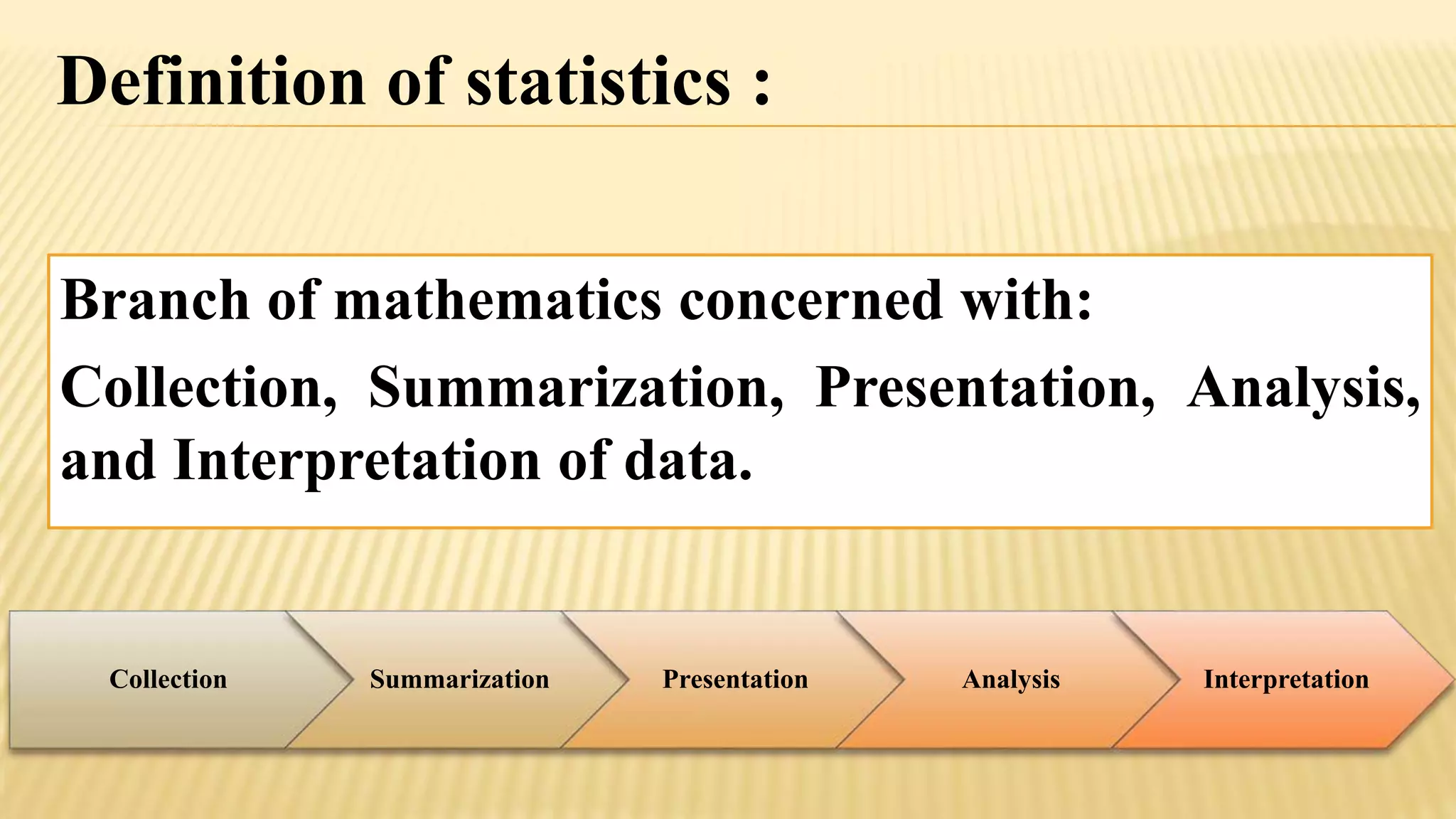
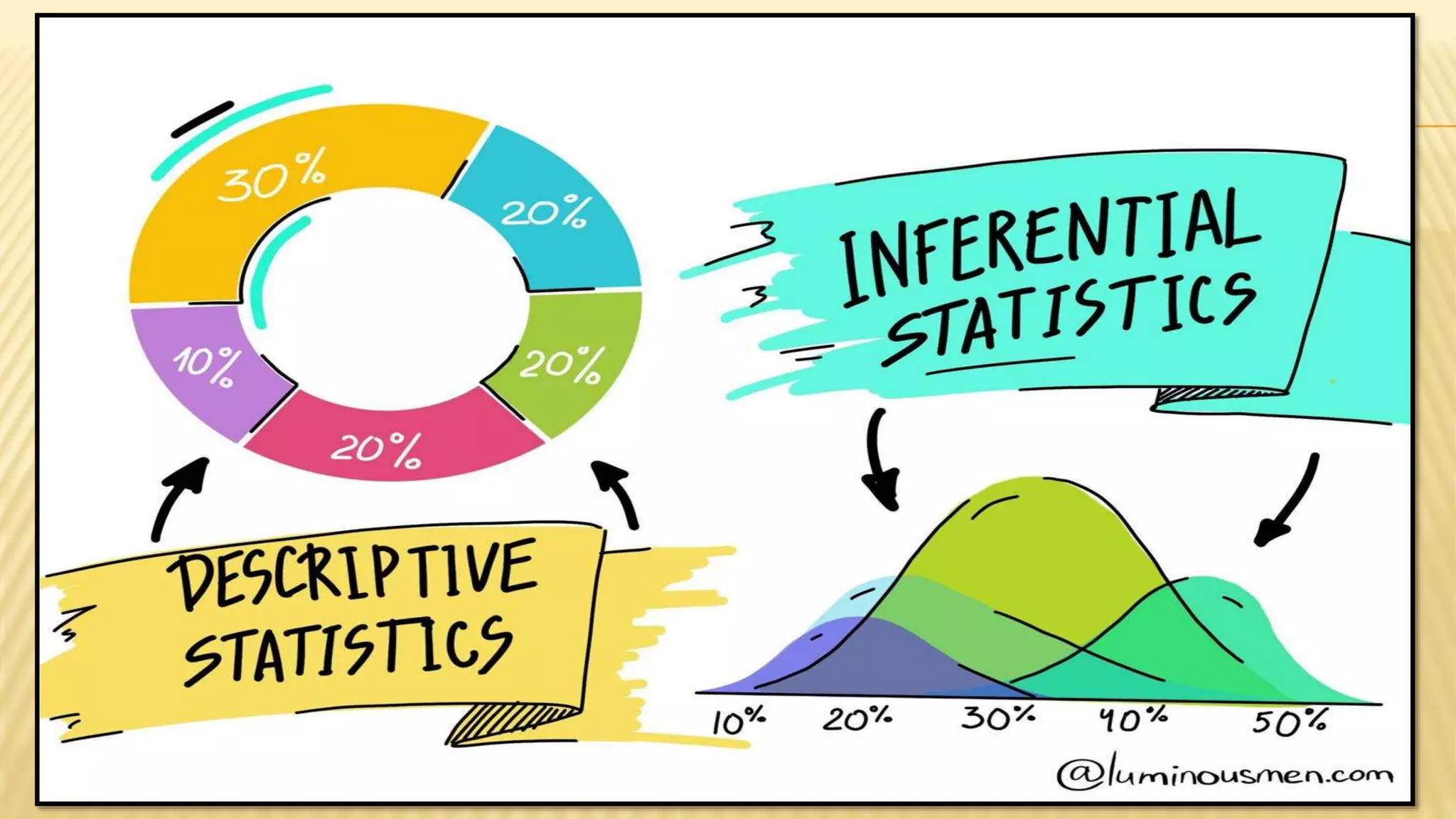
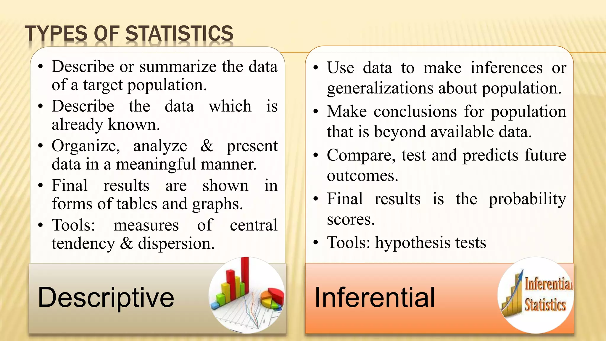
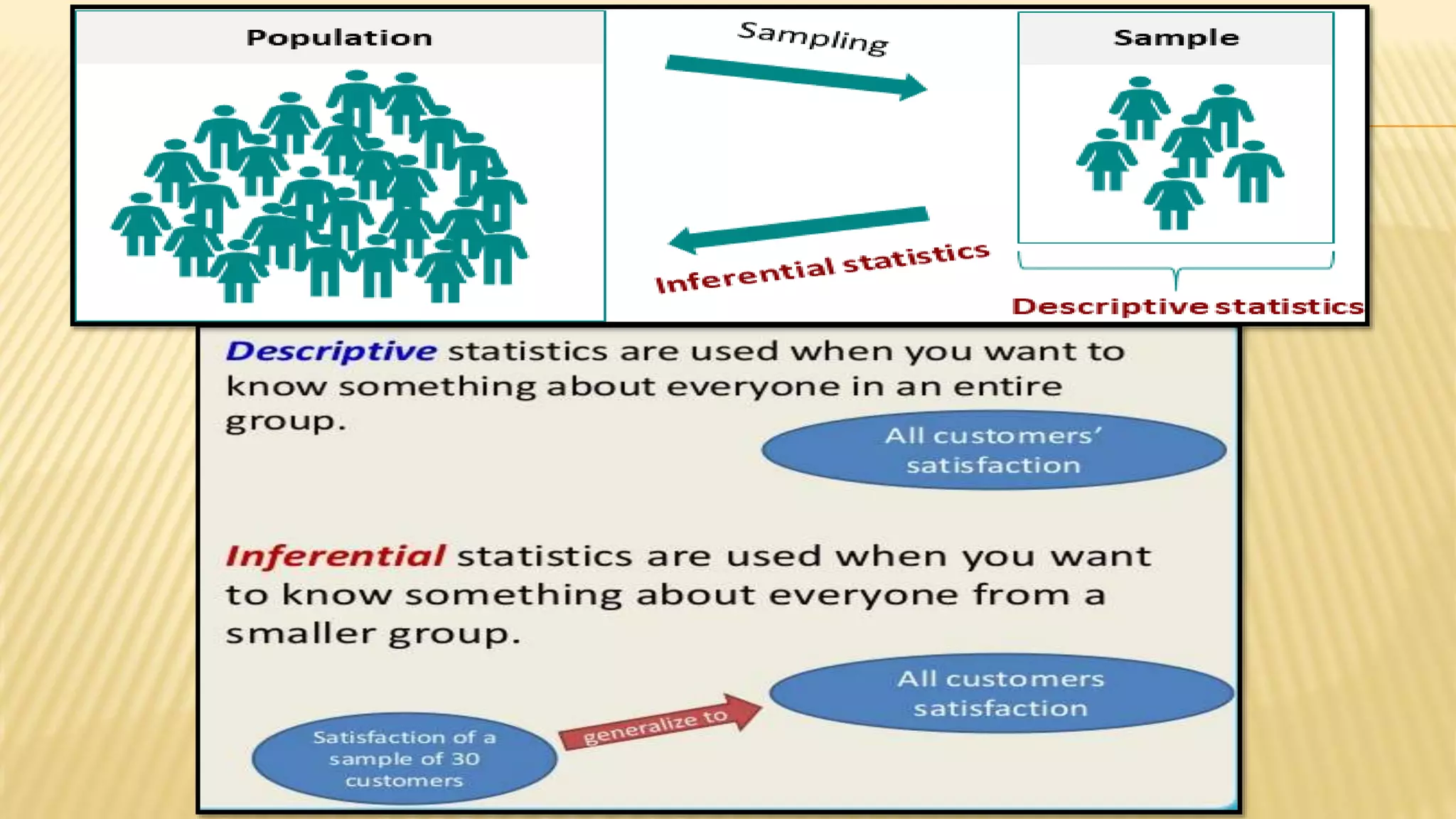
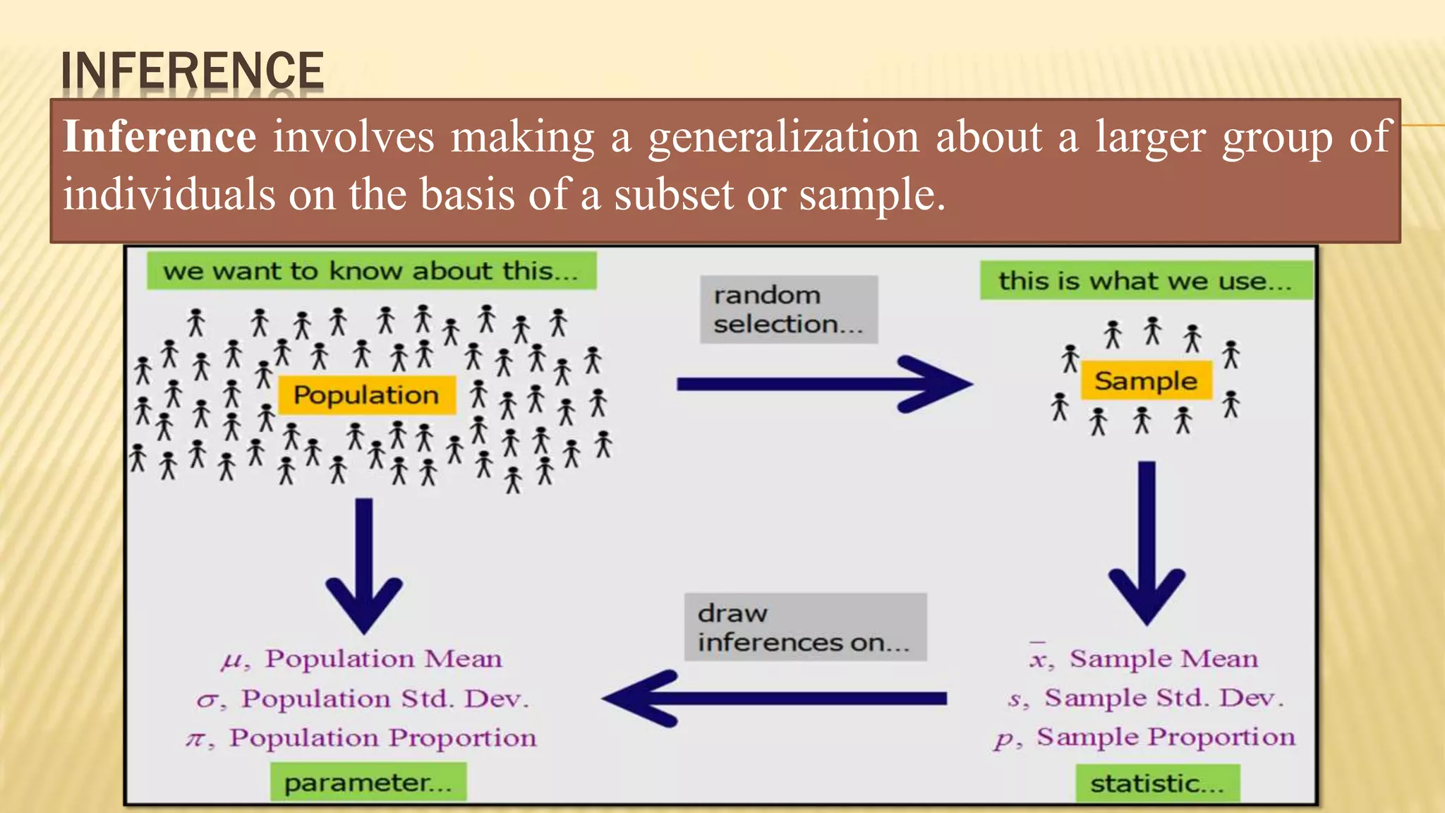
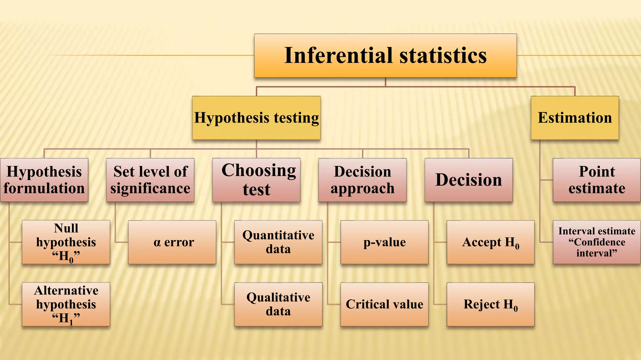
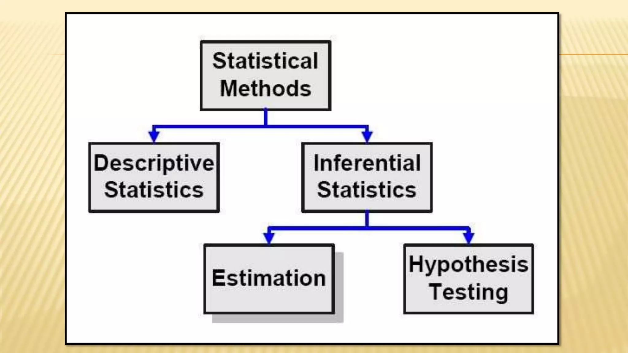
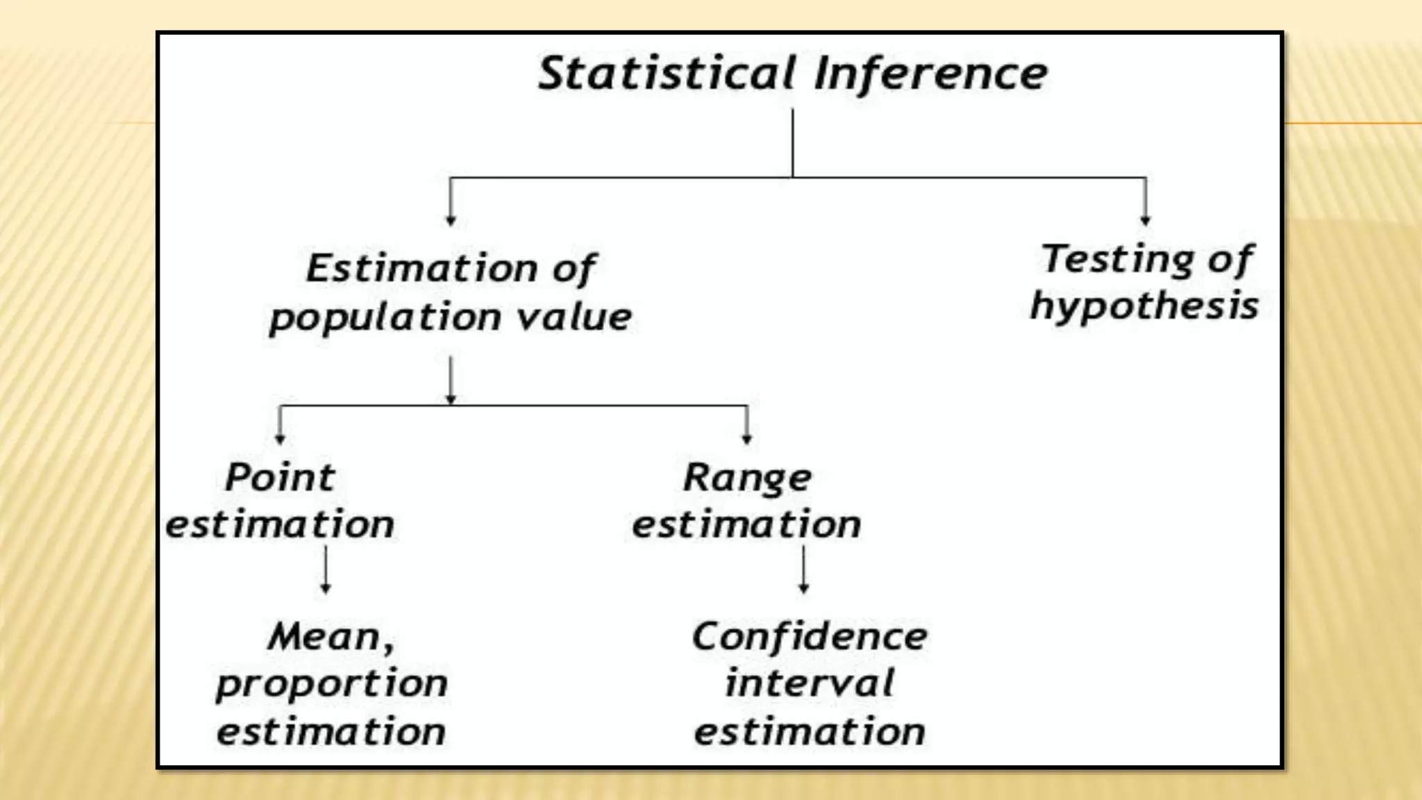
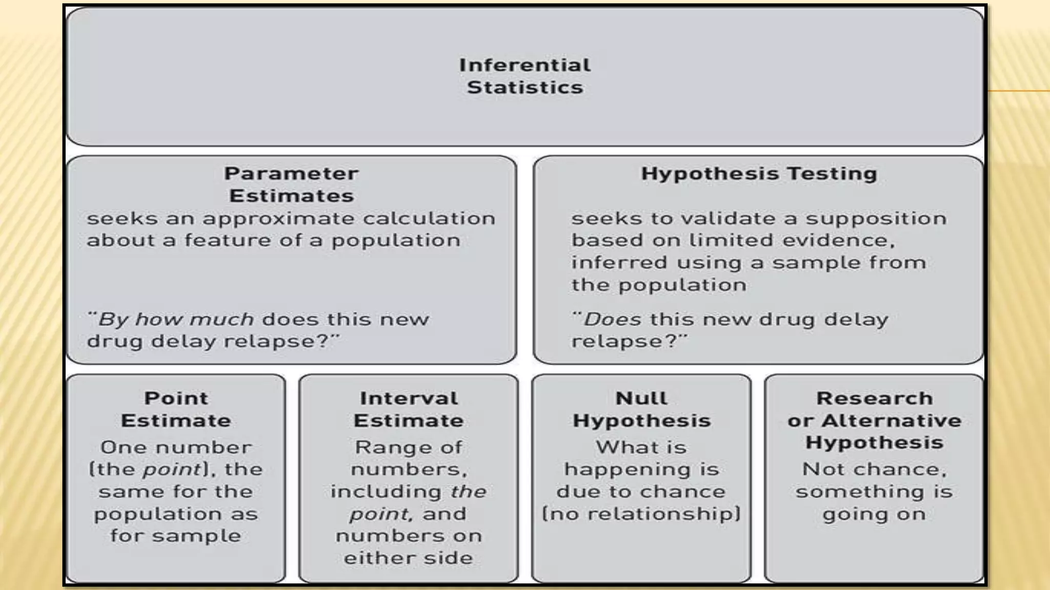
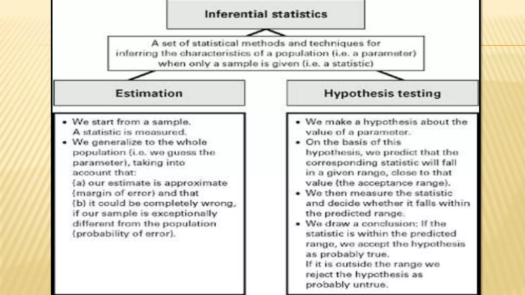
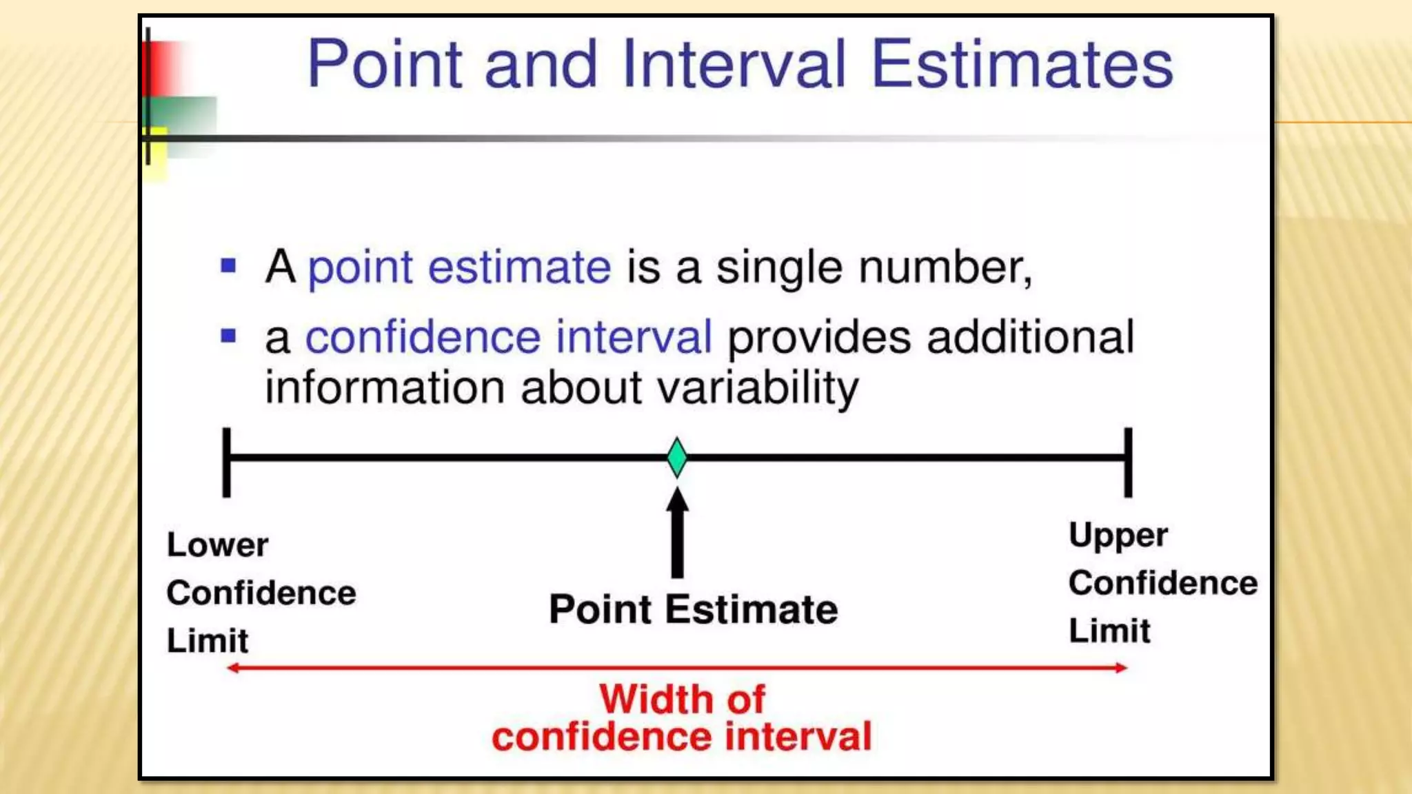
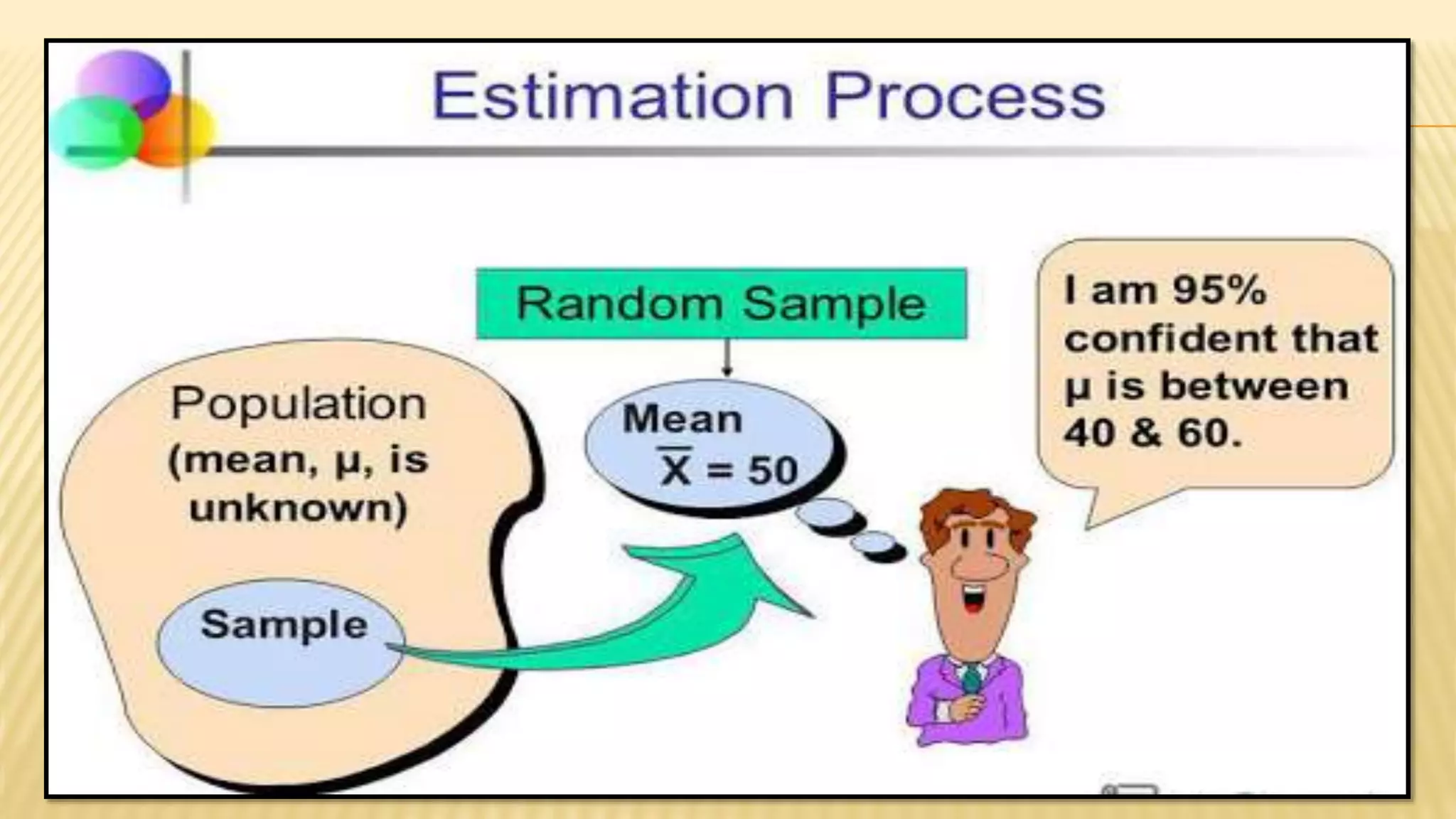
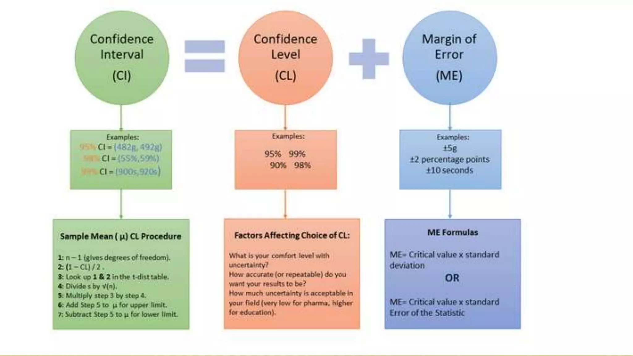
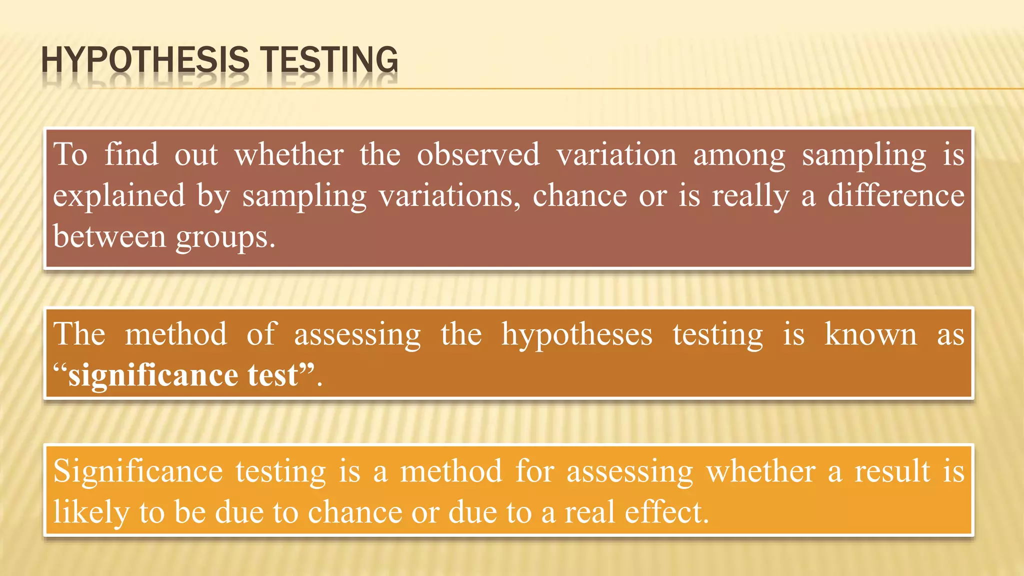
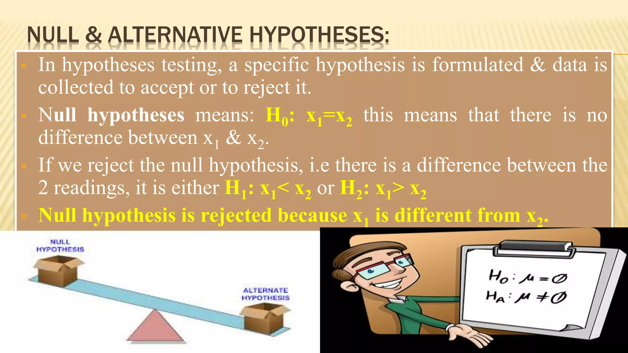
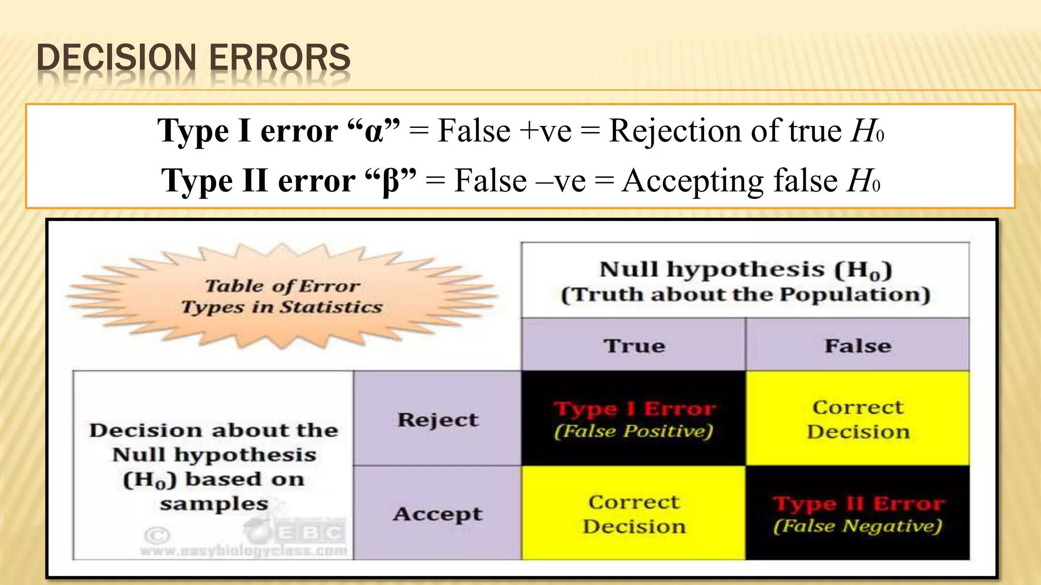
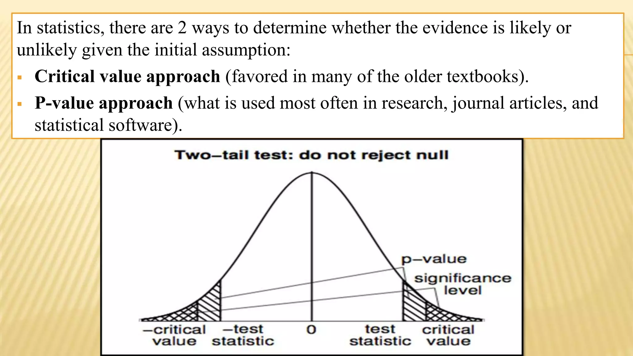
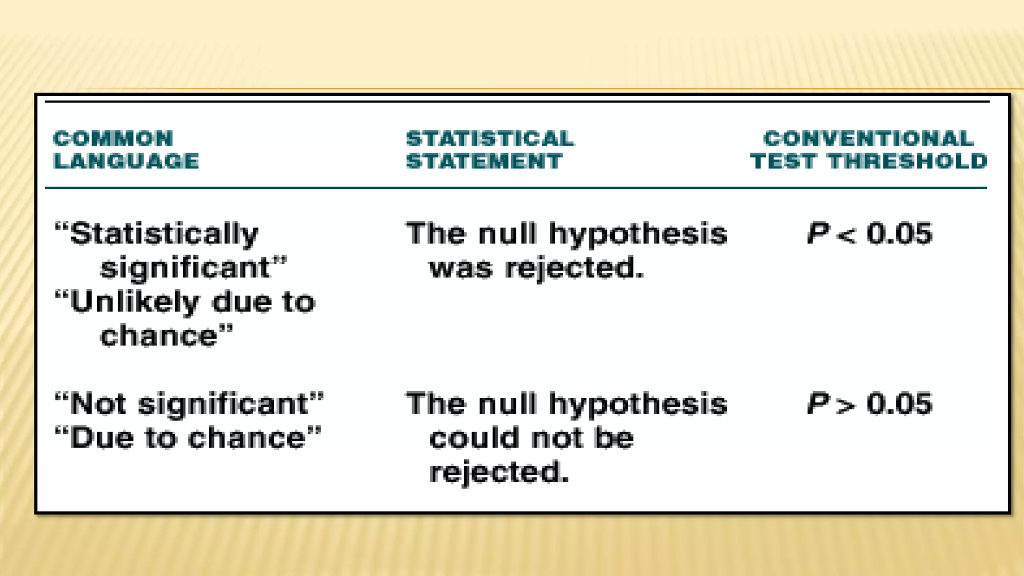
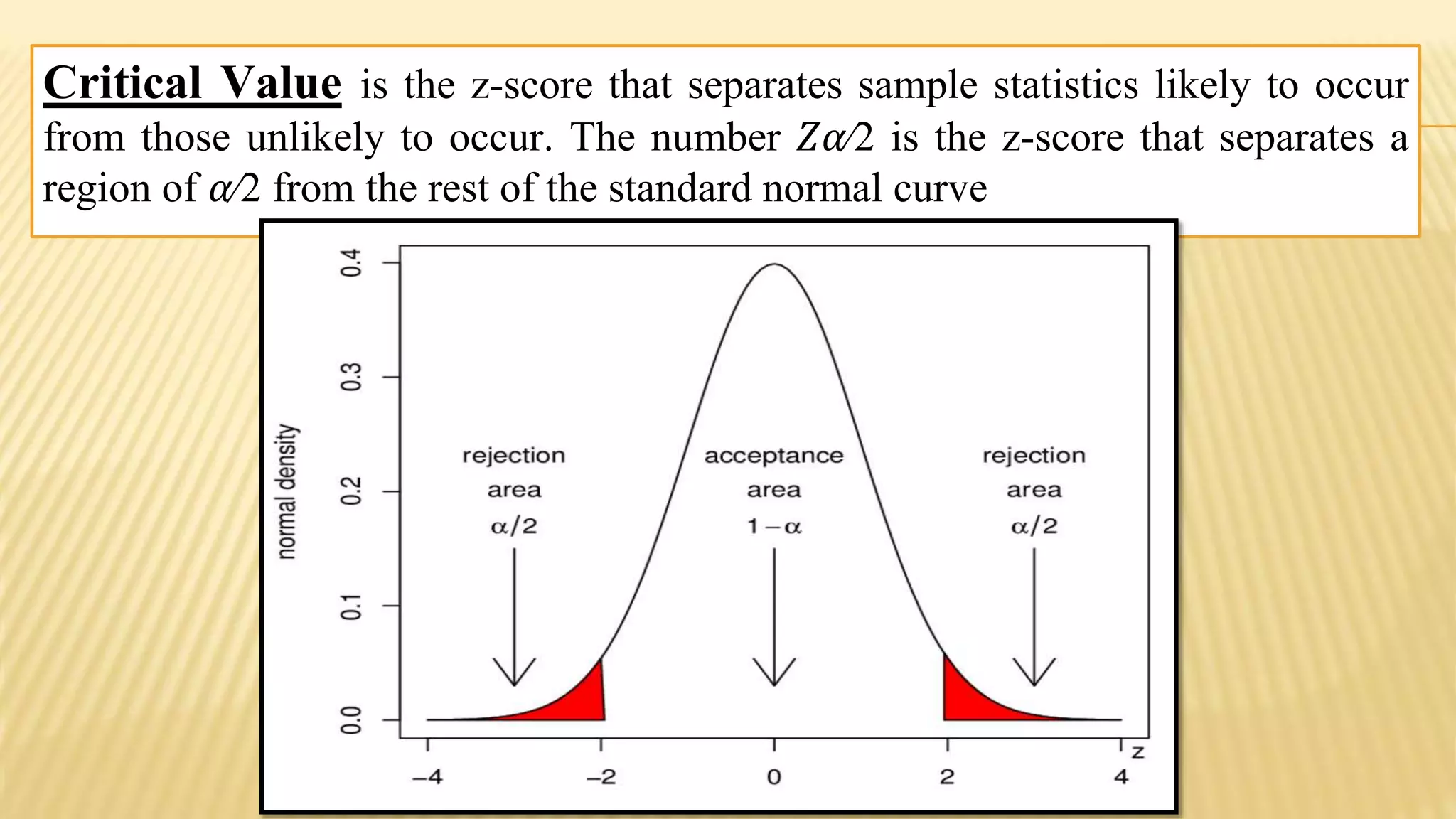
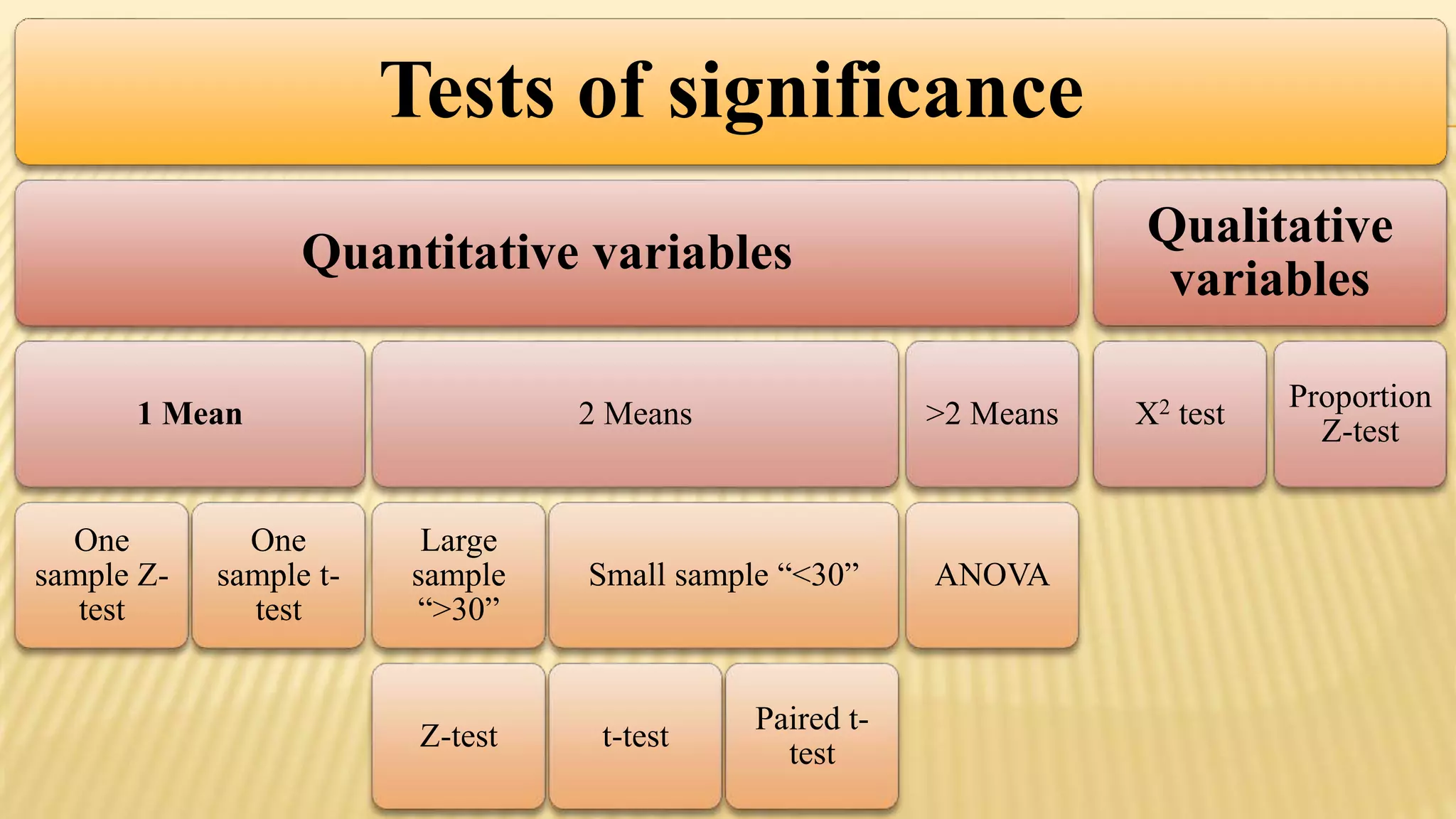
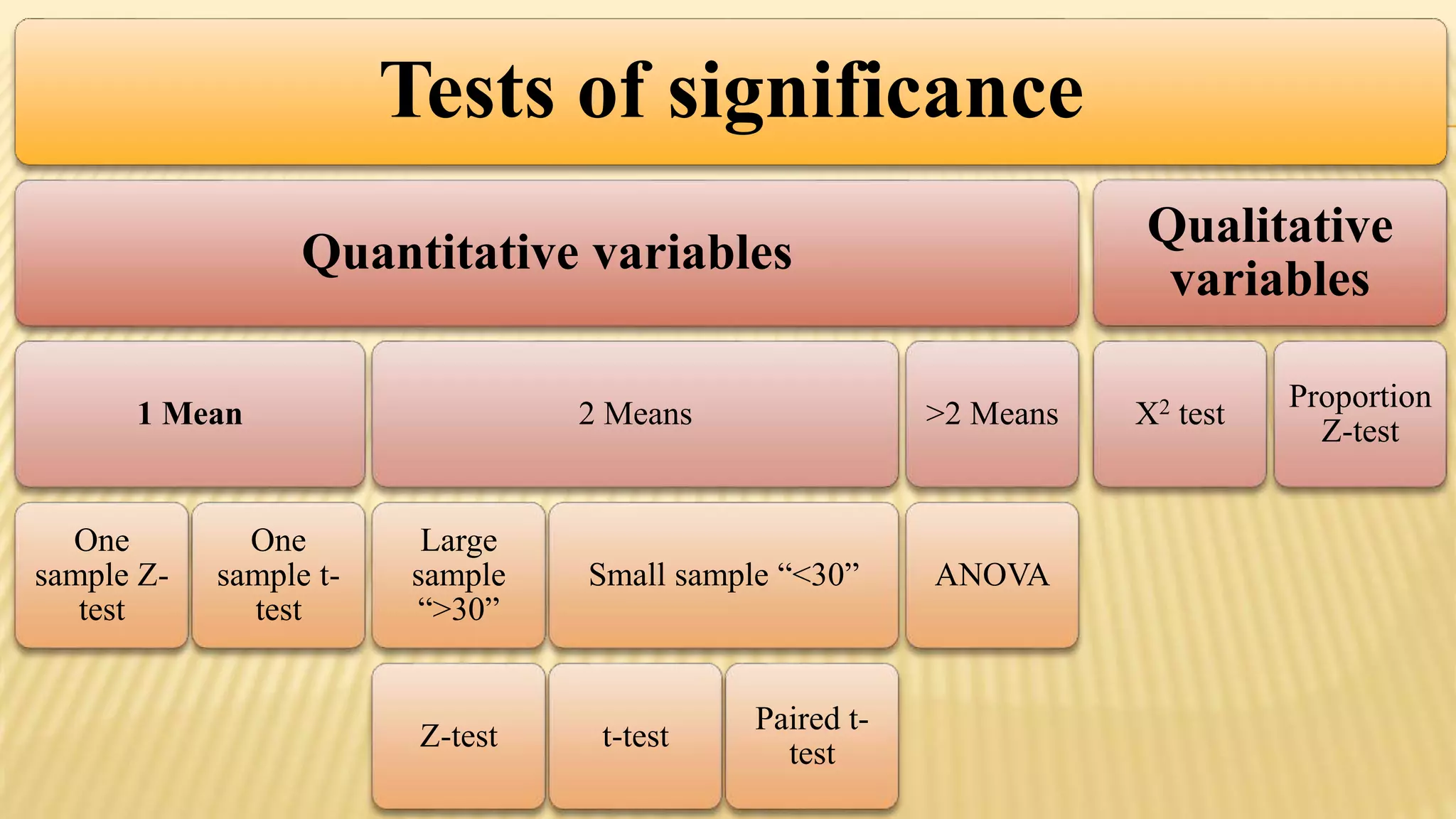
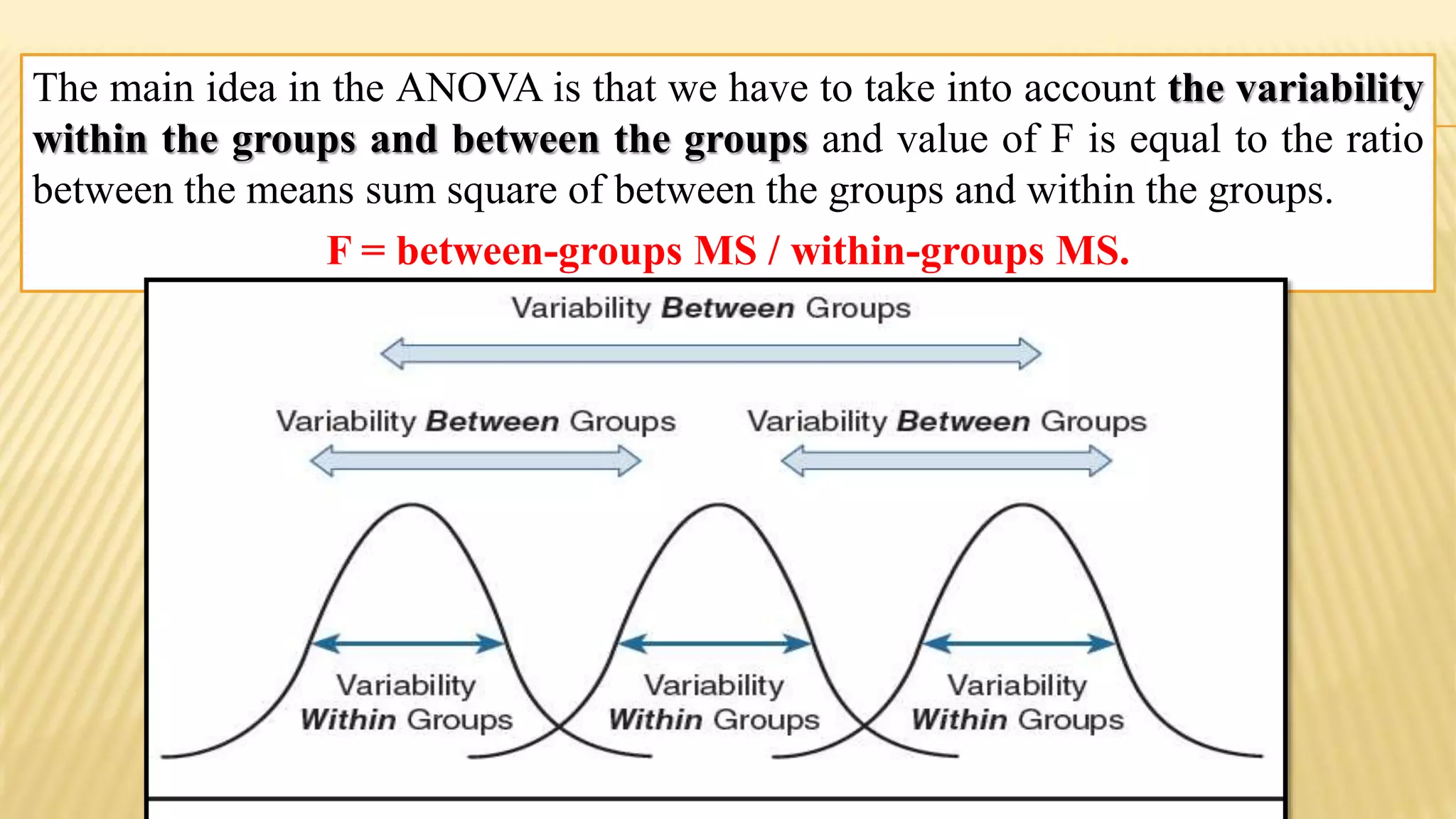
The document provides an overview of inferential statistics. It defines inferential statistics as making generalizations about a larger population based on a sample. Key topics covered include hypothesis testing, types of hypotheses, significance tests, critical values, p-values, confidence intervals, z-tests, t-tests, ANOVA, chi-square tests, correlation, and linear regression. The document aims to explain these statistical concepts and techniques at a high level.

1. INFERENTIAL STATISTICS
Dr. Dalia El-Shafei
Assist.Prof., Community Medicine Department, Zagazig University
http://www.slideshare.net/daliaelshafei

2. Definition of statistics :
Branch of mathematics concerned with:
Collection, Summarization, Presentation, Analysis,
and Interpretation of data.
Collection Summarization Presentation Analysis Interpretation

4. TYPES OF STATISTICS
• Describe or summarize the data
of a target population.
• Describe the data which is
already known.
• Organize, analyze & present
data in a meaningful manner.
• Final results are shown in
forms of tables and graphs.
• Tools: measures of central
tendency & dispersion.
Descriptive
• Use data to make inferences or
generalizations about population.
• Make conclusions for population
that is beyond available data.
• Compare, test and predicts future
outcomes.
• Final results is the probability
scores.
• Tools: hypothesis tests
Inferential

6. INFERENCE
Inference involves making a generalization about a larger group of
individuals on the basis of a subset or sample.

7. Inferential statistics
Hypothesis testing
Hypothesis
formulation
Null
hypothesis
“H0”
Alternative
hypothesis
“H1”
Set level of
significance
α error
Choosing
test
Quantitative
data
Qualitative
data
Decision
approach
p-value
Critical value
Decision
Accept H0
Reject H0
Estimation
Point
estimate
Interval estimate
“Confidence
interval”

18. CONFIDENCE LEVEL & INTERVAL “INTERVAL ESTIMATE”
Confidence
interval
“Interval
estimate”
• The range of values that is used to
estimate the true value of the
population parameter.
Confidence
Level
• The probability that the confidence
interval does, in fact, contain the
true population parameter, assuming
that the estimation process is
repeated many times (1−𝛼).

26. HYPOTHESIS TESTING
To find out whether the observed variation among sampling is
explained by sampling variations, chance or is really a difference
between groups.
The method of assessing the hypotheses testing is known as
“significance test”.
Significance testing is a method for assessing whether a result is
likely to be due to chance or due to a real effect.

27. NULL & ALTERNATIVE HYPOTHESES:
 In hypotheses testing, a specific hypothesis is formulated & data is
collected to accept or to reject it.
 Null hypotheses means: H0: x1=x2 this means that there is no
difference between x1 & x2.
 If we reject the null hypothesis, i.e there is a difference between the
2 readings, it is either H1: x1< x2 or H2: x1> x2
 Null hypothesis is rejected because x1 is different from x2.

30. Compared the smoking cessation rates for smokers randomly
assigned to use a nicotine patch versus a placebo patch.
Null hypothesis: Smoking cessation rate in nicotine patch group =
smoking cessation rate in placebo patch group.
Alternative hypothesis: Smoking cessation rate in nicotine patch
group ≠ smoking cessation rate in placebo patch group (2 tailed) OR
smoking cessation rate in nicotine patch group is higher than smoking
cessation rate in placebo patch group (1 tailed).

32. DECISION ERRORS
Type I error “α” = False +ve = Rejection of true H0
Type II error “β” = False –ve = Accepting false H0

36. In statistics, there are 2 ways to determine whether the evidence is likely or
unlikely given the initial assumption:
 Critical value approach (favored in many of the older textbooks).
 P-value approach (what is used most often in research, journal articles, and
statistical software).

37.  If the data are not consistent with the null hypotheses, the difference is
said to be “statistically significant”.
 If the data are consistent with the null hypotheses it is said that we accept
it i.e. statistically insignificant.
 In medicine, we usually consider that differences are significant if the
probability is <0.05.
 This means that if the null hypothesis is true, we shall make a wrong decision
<5 in a 100 times.

41. CRITICAL VALUE

42. CRITICAL VALUE
A point on the test distribution that is compared to the test statistic to
determine whether to reject the null hypothesis.
If the absolute value of your test statistic is greater than the
critical value, you can declare statistical significance and reject the
null hypothesis.
Critical values correspond to α, so their values become fixed when
you choose the test's α.

44. Critical Value is the z-score that separates sample statistics likely to occur
from those unlikely to occur. The number 𝑍𝛼⁄2 is the z-score that separates a
region of 𝛼⁄2 from the rest of the standard normal curve

46. TESTS OF SIGNIFICANCE

48. Tests of significance
Quantitative variables
1 Mean
One
sample Z-
test
One
sample t-
test
2 Means
Large
sample
“>30”
Z-test
Small sample “<30”
t-test
Paired t-
test
>2 Means
ANOVA
Qualitative
variables
X2 test
Proportion
Z-test

50. ANALYSIS OF QUANTITATIVE
VARIABLES

51. Tests of significance
Quantitative variables
1 Mean
One
sample Z-
test
One
sample t-
test
2 Means
Large
sample
“>30”
Z-test
Small sample “<30”
t-test
Paired t-
test
>2 Means
ANOVA
Qualitative
variables
X2 test
Proportion
Z-test

52. Z TEST OR SND
“STANDARD NORMAL DEVIATE”

54. Z TEST OR SND STANDARD NORMAL DEVIATE
 Used for Comparing 2 means of large samples (>60) using the
normal distribution.

61. Student’s t-test

63. STUDENT'S T-TEST
 Used for Comparing two means of small samples (<60) by the t
distribution instead of the normal distribution.

65. UNPAIRED T-TEST
 X1= mean of the 1st sample X2=mean of the 2nd sample
 n1= sample size of the 1st sample n2= sample size of the 2nd sample
 SD1= SD of the 1st sample SD2 = SD of the 2nd sample.
 Degree of freedom (df) = (n1+n2)-2

66. STUDENT'S T-TEST
 The value of t will be compared to values in the specific table of "t
distribution test" at the value of the degree of freedom.
 If the calculated value of t is less than that in the table, then the difference
between samples is insignificant.
 If the calculated t value is larger than that in the table so the difference is
significant i.e. the null hypothesis is rejected.

67. Big t-value
Small P-
value
Statistical
significance

68. STUDENT'S T-TEST
Calculated t (1.75) < Tabulated t (3.182), then the difference between samples is
insignificant. i.e. Null hypothesis is accepted.
Suppose that you calculate t test= 1.75
Suppose that df = 3

69. PAIRED T-TEST
Comparing repeated observation in the same individual or difference
between paired data.
The analysis is carried out using the mean & SD of the difference
between each pair.

71. ANALYSIS OF VARIANCE
(ANOVA)

72.  Used for Comparing several means.
 To compare >2 means, this can be done by use of several t-tests that can
consume more time & lead to spurious significant results. So, we must use
analysis of variance or ANOVA.

73. ANALYSIS OF VARIANCE (ANOVA)
There are two main types:
• When the subgroups to be compared are defined by just one factor
• Comparison between means of blood glucose levels among 3 groups of
diabetic patients (1st group was on insulin, 2nd group was on oral
hypoglycemic drugs, & 3rd group was on lifestyle modification)
One-way ANOVA
• When the subdivision is based upon more than one factor.
• The above-mentioned example the groups were divided into males & females.
Two-way ANOVA

74. The main idea in the ANOVA is that we have to take into account the variability
within the groups and between the groups and value of F is equal to the ratio
between the means sum square of between the groups and within the groups.
F = between-groups MS / within-groups MS.

75. ANALYSIS OF QUALITATIVE
VARIABLES

76. Tests of significance
Quantitative variables
1 Mean
One
sample Z-
test
One
sample t-
test
2 Means
Large
sample
“>30”
Z-test
Small sample “<30”
t-test
Paired t-
test
>2 Means
ANOVA
Qualitative
variables
X2 test
Proportion
Z-test

77. Chi -square test

78. CHI -SQUARE TEST
Test relationships between categorical independent variables.
Qualitative data are arranged in table formed by rows & columns.
Variables Obese Non-Obese Total
Diabetic 62 63 125
Non-diabetic 51 44 105
Total 113 107 220

79. O = Observed value in the table
E = Expected value
Expected (E) = Row total Χ Column total
Grand total
Degree of freedom =
(row - 1) (column - 1)

80. EXAMPLE HYPOTHETICAL STUDY
 Two groups of patients are treated using different spinal
manipulation techniques
 Gonstead vs. Diversified
 The presence or absence of pain after treatment is the outcome
measure.
 Two categories
 Technique used
 Pain after treatment

81. GONSTEAD VS. DIVERSIFIED EXAMPLE - RESULTS
Yes No Row Total
Gonstead 9 21 30
Diversified 11 29 40
Column Total 20 50 70
Grand Total
Technique
Pain after treatment
9 out of 30 (30%) still had pain after Gonstead treatment
and 11 out of 40 (27.5%) still had pain after Diversified,
but is this difference statistically significant?

82.  To find E for cell a (and similarly for the rest)
Yes No Row Total
Gonstead 9 21 30
Diversified 11 29 40
Column Total 20 50 70
Grand Total
Technique
Pain after treatment
Multiply row total
Times column total
Divide by grand total
FIRST FIND THE EXPECTED VALUES FOR EACH CELL
Expected (E) = Row total Χ Column total
Grand total

83.  Find E for all cells
Yes No Row Total
Gonstead
9
E = 30*20/70=8.6
21
E = 30*50/70=21.4
30
Diversified
11
E=40*20/70=11.4
29
E=40*50/70=28.6
40
Column Total 20 50 70
Grand
Total
Technique
Pain after treatment

84.  Use the Χ2
formula with each cell and then add them together
Χ2 = 0.0186 + 0.0168 + 0.0316 + 0.0056 = 0.0726
(9 - 8.6)2
8.6
(21 - 21.4)2
21.4
=
0.018
6
0.0168
(11 - 11.4)2
11.4
(29 - 28.6)2
28.6
0.031
6
0.0056

85. Evidence-based Chiropractic
Therefore, Χ
2
is not statistically significant
So, we will accept null hypothesis
Calculated χ2 value (0.0726) < Tabulated value (7.815)
at df = 1.

86. Z TEST FOR COMPARING 2
PERCENTAGES
“PROPORTION Z-TEST”

87. Z TEST FOR COMPARING 2 PERCENTAGES “PROPORTION Z-TEST”
p1=% in the 1st group. p2 = % in the 2nd group
q1=100-p1 q2=100-p2
n1= sample size of 1st group
n2=sample size of 2nd group .
Z test is significant (at 0.05 level) if the result >2.
Z= p1 – p2 /√(p1q1/n1 + p2q2/n2).

88. EXAMPLE
If the number of anemic patients in group 1 which includes 50 patients
is 5 and the number of anemic patients in group 2 which contains 60
patients is 20. if groups 1 & 2 are statistically different in prevalence of
anemia we calculate z test.
p1=5/50=10% p2=20/60=33% q1=100-10=90 q2=100-33=67
Z= 10 – 33/ √ (10x90/50 + 33x67/60)
Z= 23 / √ (18 + 36.85) Z= 23/ 7.4 Z= 3.1
So, there is statistically significant difference between percentages of
anemia in the studied groups (because Z>2).

89. CORRELATION & REGRESSION

90. CORRELATION & REGRESSION
Correlation measures the closeness of the association between 2
continuous variables, while Linear regression gives the equation of
the straight line that best describes & enables the prediction of one
variable from the other.

91. CORRELATION IS NOT CAUSATION!!!

92. LINEAR REGRESSION
Same as correlation
•Determine the relation & prediction of the
change in a variable due to changes in
other variable.
•t-test is also used for the assessment of the
level of significance.
Differ than correlation
•The independent factor has to be
specified from the dependent
variable.
•The dependent variable in linear
regression must be a continuous
one.
•Allows the prediction of dependent
variable for a particular independent
variable “But, should not be used
outside the range of original data”.

93. CORRELATION
 Measured by the correlation coefficient, r. The values of r ranges between +1
and -1.
 “1” means perfect correlation while “0” means no correlation.
 If r value is near the zero, it means weak correlation while near the one it
means strong correlation. The sign - and + denotes the direction of correlation

95. REGRESSION

96. LINEAR REGRESSION
 Used to determine the relation & prediction of the change in a
variable due to changes in another variable.
 For linear regression, the independent factor (x) must be specified
from the dependent variable (y).
 Also allows the prediction of dependent variable for a particular
independent variable

97. SCATTERPLOTS
 An X-Y graph with symbols that represent the values of 2 variables
Regression line

98. LINEAR REGRESSION
 However, regression for
prediction should not be used
outside the range of original
data.
 t-test is also used for the
assessment of the level of
significance.
 The dependent variable in
linear regression must be a
continuous one.

99. MULTIPLE LINEAR REGRESSION
 The dependency of a dependent variable on several independent
variables, not just one.
 Test of significance used is the ANOVA. (F test).

100. EXAMPLE
 If neonatal birth weight depends on these factors: gestational age, length of
baby and head circumference. Each factor correlates significantly with baby
birth weight (i.e has +ve linear correlation).
 We can do multiple regression analysis to obtain a mathematical equation by
which we can predict the birth weight of any neonate if we know the values of
these factors.