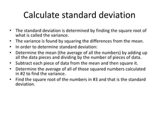
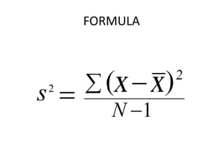
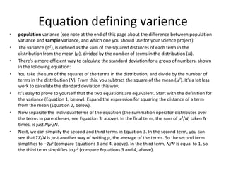
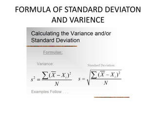
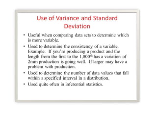
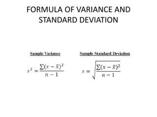
A teacher calculated the standard deviation of test scores to see how close students scored to the mean grade of 65%. She found the standard deviation was high, indicating outliers pulled the mean down. An employer also calculated standard deviation to analyze salary fairness, finding it slightly high due to long-time employees making more. Standard deviation measures dispersion from the mean, with low values showing close grouping and high values showing a wider spread. It is calculated using the variance formula of summing the squared differences from the mean divided by the number of values.

1. Standard Deviation
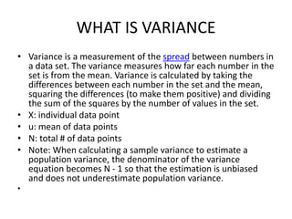
In statistics, the standard deviation (SD, also represented by the Greek letter
sigma σ or the Latin letter s) is a measure that is used to quantify the amount
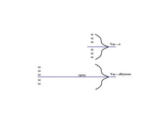
of variation or dispersion of a set of data values.[1] A low standard deviation
indicates that the data points tend to be close to the mean (also called the
expected value) of the set, while a high standard deviation indicates that the
data points are spread out over a wider range of values.
The standard deviation of a random variable, statistical population, data set,
or probability distribution is the square root of its variance. It is algebraically
simpler, though in practice less robust, than the average absolute
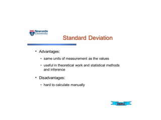
deviation.[2][3] A useful property of the standard deviation is that, unlike the
variance, it is expressed in the same units as the data. There are also other
measures of deviation from the norm, including average absolute deviation,
which provide different mathematical properties from standard deviation.[4]
In addition to expressing the variability of a population, the standard deviation
is commonly used to measure confidence in statistical conclusions. For
example, the margin of error in polling data is determined by calculating the
expected standard deviation in the results if the same poll were to be

2. conducted multiple times. This derivation of a standard deviation is often called the
"standard error" of the estimate or "standard error of the mean" when referring to a
mean. It is computed as the standard deviation of all the means that would be computed
from that population if an infinite number of samples were drawn and a mean for each
sample were computed.
It is very important to note that the standard deviation of a population and the standard
error of a statistic derived from that population (such as the mean) are quite different but
related (related by the inverse of the square root of the number of observations). The
reported margin of error of a poll is computed from the standard error of the mean (or
alternatively from the product of the standard deviation of the population and the inverse
of the square root of the sample size, which is the same thing) and is typically about twice
the standard deviation—the half-width of a 95 percent confidence interval.
In science, many researchers report the standard deviation of experimental data, and only
effects that fall much farther than two standard deviations away from what would have
been expected are considered statistically significant—normal random error or variation in
the measurements is in this way distinguished from likely genuine effects or associations.
The standard deviation is also important in finance, where the standard deviation on the
rate of return on an investment is a measure of the volatility of the investment.
When only a sample of data from a population is available, the term standard deviation of
the sample or sample standard deviation can refer to either the above-mentioned
quantity as applied to those data or to a modified quantity that is an unbiased estimate of
the population standard deviation (the standard deviation of the entire population).

3. USE OF STANDARD DEVIATON
• Some examples of situations in which standard deviation might help to understand
the value of the data:
• A class of students took a math test. Their teacher found that the mean score on the
test was an 85%. She then calculated the standard deviation of the other test scores
and found a very small standard deviation which suggested that most students scored
very close to 85%.
• A dog walker wants to determine if the dogs on his route are close in weight or not
close in weight. He takes the average of the weight of all ten dogs. He then calculates
the variance, and then the standard deviation. His standard deviation is extremely
high. This suggests that the dogs are of many various weights, or that he has a few
dogs whose weights are outliers that are skewing the data.
• A market researcher is analyzing the results of a recent customer survey. He wants to
have some measure of the reliability of the answers received in the survey in order to
predict how a larger group of people might answer the same questions. A low
standard deviation shows that the answers are very projectable to a larger group of
people.
• A weather reporter is analyzing the high temperature forecasted for a series of dates
versus the actual high temperature recorded on each date. A low standard deviation
would show a reliable weather forecast.

4. A class of students took a test in Language Arts. The teacher determines that the mean
grade on the exam is a 65%. She is concerned that this is very low, so she determines the
standard deviation to see if it seems that most students scored close to the mean, or not.
The teacher finds that the standard deviation is high. After closely examining all of the
tests, the teacher is able to determine that several students with very low scores were the
outliers that pulled down the mean of the entire class’s scores.
An employer wants to determine if the salaries in one department seem fair for all
employees, or if there is a great disparity. He finds the average of the salaries in that
department and then calculates the variance, and then the standard deviation. The
employer finds that the standard deviation is slightly higher than he expected, so he
examines the data further and finds that while most employees fall within a similar pay
bracket, three loyal employees who have been in the department for 20 years or more, far
longer than the others, are making far more due to their longevity with the company. Doing
the analysis helped the employer to understand the range of salaries of the people in the
department.

5. FORMULA OF STANDARD DEVIATION
• The sample standard deviation of the metabolic rate
for the female fulmars is calculated as follows. The
formula for the sample standard deviation is
• s = ∑ i = 1 N ( x i − x ¯ ) 2 N − 1 . {displaystyle s={sqrt
{frac {sum _{i=1}^{N}(x_{i}-{overline {x}})^{2}}{N-
1}}}.} where { x 1 , x 2 , … , x N } {displaystyle
scriptstyle {x_{1},,x_{2},,ldots ,,x_{N}}} are the
observed values of the sample items, x ¯ {displaystyle
scriptstyle {overline {x}}} is the mean value of these
observations, and N is the number of observations in
the sample.

6. Calculate standard deviation
• The standard deviation is determined by finding the square root of
what is called the variance.
• The variance is found by squaring the differences from the mean.
• In order to determine standard deviation:
• Determine the mean (the average of all the numbers) by adding up
all the data pieces and dividing by the number of pieces of data.
• Subtract each piece of data from the mean and then square it.
• Determine the average of all of those squared numbers calculated
in #2 to find the variance.
• Find the square root of the numbers in #3 and that is the standard
deviation.

7. What standards bring
• Improved market access as a result of increased competitiveness and efficiency,
reduced trading costs, simplified contractual agreements, and increased quality.
• Better relations with suppliers and clients derived from the improved safety of
consumers.
• An immense value for the competitiveness of enterprises working in transport,
machinery, electro-technical products, or telecommunications.
• Easier introduction of innovative products provided by interoperability between
new and existing products, services, and processes - for example in the field of
eco-design, smart grids, energy efficiency of buildings, nanotechnologies, security,
and eMobility.
• Help to bridge the gap between research and marketable products or services.

9. VARIENCE
• Variance is a statistical measure that tells us
how measured data vary from the average
value of the set of data.
• In other words, variance is the mean of the
squares of the deviations from the arithmetic
mean of a data set.

10. • Variance measures how far a data set is spread out. The
technical definition is “The average of the squared
differences from the mean,” but all it really does is to give
you a very general idea of the spread of your data. A value
of zero means that there is no variability; All the numbers
in the data set are the same.
• The data set 12, 12, 12, 12, 12 has a var. of zero (the
numbers are identical).
• The data set 12, 12, 12, 12, 13 has a var. of 0.167; a small
change in the numbers equals a very small var.
• The data set 12, 12, 12, 12, 13,013 has a var. of 28171000; a
large change in the numbers equals a very large number.

11. WHAT IS VARIANCE
• Variance is a measurement of the spread between numbers in
a data set. The variance measures how far each number in the
set is from the mean. Variance is calculated by taking the
differences between each number in the set and the mean,
squaring the differences (to make them positive) and dividing
the sum of the squares by the number of values in the set.
• X: individual data point
• u: mean of data points
• N: total # of data points
• Note: When calculating a sample variance to estimate a
population variance, the denominator of the variance
equation becomes N - 1 so that the estimation is unbiased
and does not underestimate population variance.
•

13. FORMULA

16. Equation defining varience
• population variance (see note at the end of this page about the difference between population
variance and sample variance, and which one you should use for your science project):
• The variance (σ2), is defined as the sum of the squared distances of each term in the
distribution from the mean (μ), divided by the number of terms in the distribution (N).
• There's a more efficient way to calculate the standard deviation for a group of numbers, shown
in the following equation:
• You take the sum of the squares of the terms in the distribution, and divide by the number of
terms in the distribution (N). From this, you subtract the square of the mean (μ2). It's a lot less
work to calculate the standard deviation this way.
• It's easy to prove to yourself that the two equations are equivalent. Start with the definition for
the variance (Equation 1, below). Expand the expression for squaring the distance of a term
from the mean (Equation 2, below).
• Now separate the individual terms of the equation (the summation operator distributes over
the terms in parentheses, see Equation 3, above). In the final term, the sum of μ2/N, taken N
times, is just Nμ2/N.
• Next, we can simplify the second and third terms in Equation 3. In the second term, you can
see that ΣX/N is just another way of writing μ, the average of the terms. So the second term
simplifies to −2μ2 (compare Equations 3 and 4, above). In the third term, N/N is equal to 1, so
the third term simplifies to μ2 (compare Equations 3 and 4, above).

17. DIFFERENCE BETWEEN STANDARD
DEVIATON AND VARIANCE
• The standard deviation is the square root of the
variance. The standard deviation is expressed in
the same units as the mean is, whereas the
variance is expressed in squared units, but for
looking at a distribution, you can use either just
so long as you are clear about what you are
using. For example, a Normal distribution with
mean = 10 and sd = 3 is exactly the same thing
as a Normal distribution with mean = 10 and
variance = 9.

18. FORMULA OF STANDARD DEVIATON
AND VARIENCE

20. FORMULA OF VARIANCE AND
STANDARD DEVIATION