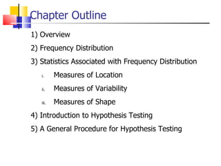
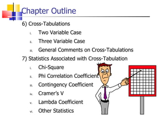
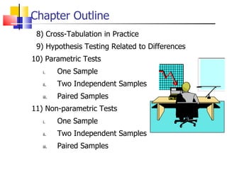
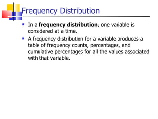
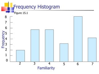
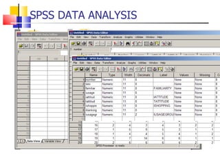
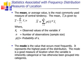
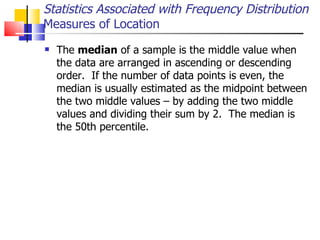
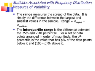
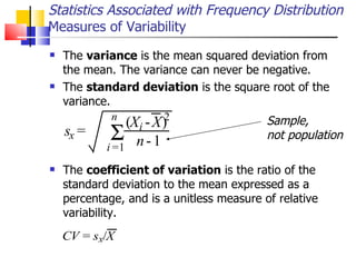
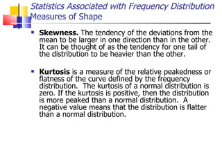
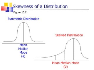
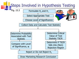
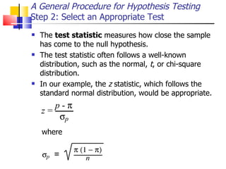
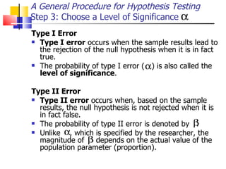
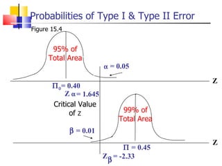
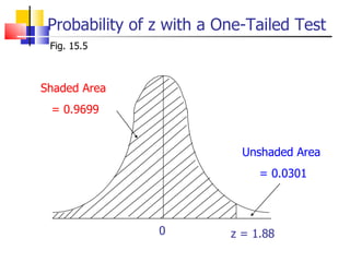
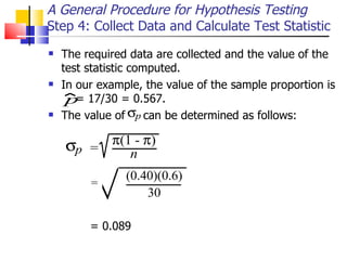
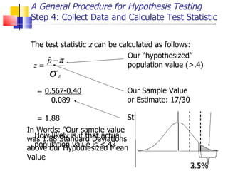
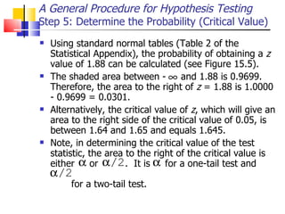
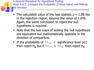
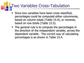
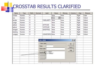
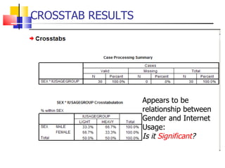
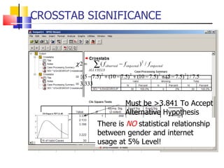
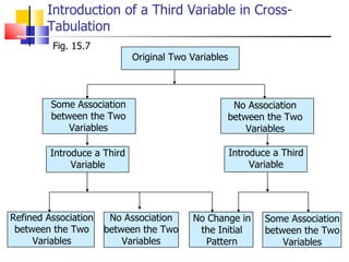
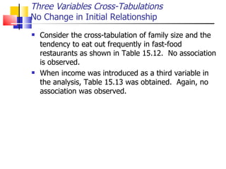
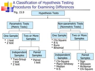
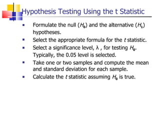
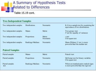
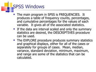
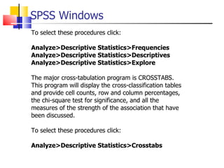
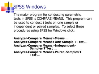
The document outlines the steps for conducting frequency distribution, cross-tabulation, and hypothesis testing analyses. It discusses measuring location, variability, and shape in frequency distributions. Cross-tabulation involves analyzing two or more variables simultaneously through tables. Hypothesis testing follows general steps including formulating hypotheses, selecting a test, determining significance levels, collecting data, and making conclusions.

1. Frequency Distribution, Cross-Tabulation, and Hypothesis Testing

2. Chapter Outline 1) Overview 2) Frequency Distribution 3) Statistics Associated with Frequency Distribution Measures of Location Measures of Variability Measures of Shape 4) Introduction to Hypothesis Testing 5) A General Procedure for Hypothesis Testing

3. Chapter Outline 6) Cross-Tabulations Two Variable Case Three Variable Case General Comments on Cross-Tabulations 7) Statistics Associated with Cross-Tabulation Chi-Square Phi Correlation Coefficient Contingency Coefficient Cramer’s V Lambda Coefficient Other Statistics

4. Chapter Outline 8) Cross-Tabulation in Practice 9) Hypothesis Testing Related to Differences 10) Parametric Tests One Sample Two Independent Samples Paired Samples 11) Non-parametric Tests One Sample Two Independent Samples Paired Samples

5. Chapter Outline 12) Internet and Computer Applications 13) Focus on Burke 14) Summary 15) Key Terms and Concepts

6. Internet Usage Data Respondent Sex Familiarity Internet Attitude Toward Usage of Internet Number Usage Internet Technology Shopping Banking 1 1.00 7.00 14.00 7.00 6.00 1.00 1.00 2 2.00 2.00 2.00 3.00 3.00 2.00 2.00 3 2.00 3.00 3.00 4.00 3.00 1.00 2.00 4 2.00 3.00 3.00 7.00 5.00 1.00 2.00 5 1.00 7.00 13.00 7.00 7.00 1.00 1.00 6 2.00 4.00 6.00 5.00 4.00 1.00 2.00 7 2.00 2.00 2.00 4.00 5.00 2.00 2.00 8 2.00 3.00 6.00 5.00 4.00 2.00 2.00 9 2.00 3.00 6.00 6.00 4.00 1.00 2.00 10 1.00 9.00 15.00 7.00 6.00 1.00 2.00 11 2.00 4.00 3.00 4.00 3.00 2.00 2.00 12 2.00 5.00 4.00 6.00 4.00 2.00 2.00 13 1.00 6.00 9.00 6.00 5.00 2.00 1.00 14 1.00 6.00 8.00 3.00 2.00 2.00 2.00 15 1.00 6.00 5.00 5.00 4.00 1.00 2.00 16 2.00 4.00 3.00 4.00 3.00 2.00 2.00 17 1.00 6.00 9.00 5.00 3.00 1.00 1.00 18 1.00 4.00 4.00 5.00 4.00 1.00 2.00 19 1.00 7.00 14.00 6.00 6.00 1.00 1.00 20 2.00 6.00 6.00 6.00 4.00 2.00 2.00 21 1.00 6.00 9.00 4.00 2.00 2.00 2.00 22 1.00 5.00 5.00 5.00 4.00 2.00 1.00 23 2.00 3.00 2.00 4.00 2.00 2.00 2.00 24 1.00 7.00 15.00 6.00 6.00 1.00 1.00 25 2.00 6.00 6.00 5.00 3.00 1.00 2.00 26 1.00 6.00 13.00 6.00 6.00 1.00 1.00 27 2.00 5.00 4.00 5.00 5.00 1.00 1.00 28 2.00 4.00 2.00 3.00 2.00 2.00 2.00 29 1.00 4.00 4.00 5.00 3.00 1.00 2.00 30 1.00 3.00 3.00 7.00 5.00 1.00 2.00 Table 15.1

7. Frequency Distribution In a frequency distribution , one variable is considered at a time. A frequency distribution for a variable produces a table of frequency counts, percentages, and cumulative percentages for all the values associated with that variable.

8. Frequency Distribution of Familiarity with the Internet Table 15.2

9. Frequency Histogram Figure 15.1 2 3 4 5 6 7 0 7 4 3 2 1 6 5 Frequency Familiarity 8

10. SPSS DATA ANALYSIS

11. The mean , or average value, is the most commonly used measure of central tendency. The mean, ,is given by Where, X i = Observed values of the variable X n = Number of observations (sample size) p(i)= Probability of x i The mode is the value that occurs most frequently. It represents the highest peak of the distribution. The mode is a good measure of location when the variable is inherently categorical or has otherwise been grouped into categories. Statistics Associated with Frequency Distribution Measures of Location X = X i / n  i = 1 n X

12. The median of a sample is the middle value when the data are arranged in ascending or descending order. If the number of data points is even, the median is usually estimated as the midpoint between the two middle values – by adding the two middle values and dividing their sum by 2. The median is the 50th percentile. Statistics Associated with Frequency Distribution Measures of Location

13. The range measures the spread of the data. It is simply the difference between the largest and smallest values in the sample. Range = X largest – X smallest. The interquartile range is the difference between the 75th and 25th percentile. For a set of data points arranged in order of magnitude, the p th percentile is the value that has p% of the data points below it and (100 - p)% above it. Statistics Associated with Frequency Distribution Measures of Variability

14. The variance is the mean squared deviation from the mean. The variance can never be negative. The standard deviation is the square root of the variance. The coefficient of variation is the ratio of the standard deviation to the mean expressed as a percentage, and is a unitless measure of relative variability. Statistics Associated with Frequency Distribution Measures of Variability s x = ( X i - X ) 2 n - 1   i = 1 n Sample, not population

15. Skewness. The tendency of the deviations from the mean to be larger in one direction than in the other. It can be thought of as the tendency for one tail of the distribution to be heavier than the other. Kurtosis is a measure of the relative peakedness or flatness of the curve defined by the frequency distribution. The kurtosis of a normal distribution is zero. If the kurtosis is positive, then the distribution is more peaked than a normal distribution. A negative value means that the distribution is flatter than a normal distribution. Statistics Associated with Frequency Distribution Measures of Shape

16. Skewness of a Distribution Figure 15.2 Skewed Distribution Symmetric Distribution Mean Median Mode (a) Mean Median Mode (b)

17. Steps Involved in Hypothesis Testing Fig. 15.3 Draw Marketing Research Conclusion Formulate H 0 and H 1 Select Appropriate Test Choose Level of Significance Determine Probability Associated with Test Statistic Determine Critical Value of Test Statistic TSCR Determine if TSCR falls into (Non) Rejection Region Compare with Level of Significance,  Reject or Do not Reject H 0 Collect Data and Calculate Test Statistic

18. A General Procedure for Hypothesis Testing Step 1: Formulate the Hypothesis A null hypothesis is a statement of the status quo, one of no difference or no effect. If the null hypothesis is not rejected, no changes will be made. An alternative hypothesis is one in which some difference or effect is expected. Accepting the alternative hypothesis will lead to changes in opinions or actions. The null hypothesis refers to a specified value of the population parameter (e.g., ), not a sample statistic (e.g., ).

19. A null hypothesis may be rejected, but it can never be accepted based on a single test. In classical hypothesis testing, there is no way to determine whether the null hypothesis is true. In marketing research, the null hypothesis is formulated in such a way that its rejection leads to the acceptance of the desired conclusion. The alternative hypothesis represents the conclusion for which evidence is sought. A General Procedure for Hypothesis Testing Step 1: Formulate the Hypothesis :  > 0 . 40 H 1

20. The test of the null hypothesis is a one-tailed test , because the alternative hypothesis is expressed directionally. If that is not the case, then a two-tailed test would be required, and the hypotheses would be expressed as: A General Procedure for Hypothesis Testing Step 1: Formulate the Hypothesis H 0 :  = 0 . 4 0 :   0 . 4 0 Generally limited to production measures for Q.C. Purposes H 1

21. The test statistic measures how close the sample has come to the null hypothesis. The test statistic often follows a well-known distribution, such as the normal, t , or chi-square distribution. In our example, the z statistic, which follows the standard normal distribution, would be appropriate. A General Procedure for Hypothesis Testing Step 2: Select an Appropriate Test where

22. Type I Error Type I error occurs when the sample results lead to the rejection of the null hypothesis when it is in fact true. The probability of type I error ( ) is also called the level of significance . Type II Error Type II error occurs when, based on the sample results, the null hypothesis is not rejected when it is in fact false. The probability of type II error is denoted by . Unlike , which is specified by the researcher, the magnitude of depends on the actual value of the population parameter (proportion). A General Procedure for Hypothesis Testing Step 3: Choose a Level of Significance

23. Power of a Test The power of a test is the probability (1 - ) of rejecting the null hypothesis when it is false and should be rejected. Although is unknown, it is related to . An extremely low value of (e.g., = 0.001) will result in intolerably high errors. So it is necessary to balance the two types of errors. A General Procedure for Hypothesis Testing Step 3: Choose a Level of Significance

24. Probabilities of Type I & Type II Error Figure 15.4 99% of Total Area Critical Value of Z   = 0.40  = 0.45  = 0.01 = 1.645 Z  = -2.33 Z  Z Z 95% of Total Area  = 0.05

25. Probability of z with a One-Tailed Test Unshaded Area = 0.0301 Fig. 15.5 Shaded Area = 0.9699 z = 1.88 0

26. The required data are collected and the value of the test statistic computed. In our example, the value of the sample proportion is = 17/30 = 0.567. The value of can be determined as follows: A General Procedure for Hypothesis Testing Step 4: Collect Data and Calculate Test Statistic = = 0.089

27. A General Procedure for Hypothesis Testing Step 4: Collect Data and Calculate Test Statistic The test statistic z can be calculated as follows: = 0.567-0.40 0.089 = 1.88 In Words: “Our sample value was 1.88 Standard Deviations above our Hypothesized Mean Value How likely is it that actual population value is <.4? Our “hypothesized” population value (>.4) Our Sample Value or Estimate: 17/30 Std Error Estimate 3.1% 2.5%

28. Using standard normal tables (Table 2 of the Statistical Appendix), the probability of obtaining a z value of 1.88 can be calculated (see Figure 15.5). The shaded area between - and 1.88 is 0.9699. Therefore, the area to the right of z = 1.88 is 1.0000 - 0.9699 = 0.0301. Alternatively, the critical value of z , which will give an area to the right side of the critical value of 0.05, is between 1.64 and 1.65 and equals 1.645. Note, in determining the critical value of the test statistic, the area to the right of the critical value is either or . It is for a one-tail test and for a two-tail test. A General Procedure for Hypothesis Testing Step 5: Determine the Probability (Critical Value)

29. If the probability associated with the calculated or observed value of the test statistic ( )is less than the level of significance ( ), the null hypothesis is rejected. The probability associated with the calculated or observed value of the test statistic is 0.0301. This is the probability of getting a p value of 0.567 when = 0.40. This is less than the level of significance of 0.05. Hence, the null hypothesis is rejected. Alternatively, if the calculated value of the test statistic is greater than the critical value of the test statistic ( ), the null hypothesis is rejected. A General Procedure for Hypothesis Testing Steps 6 & 7: Compare the Probability (Critical Value) and Making the Decision 

30. The calculated value of the test statistic z = 1.88 lies in the rejection region, beyond the value of 1.645. Again, the same conclusion to reject the null hypothesis is reached. Note that the two ways of testing the null hypothesis are equivalent but mathematically opposite in the direction of comparison. If the probability of < significance level ( ) then reject H 0 but if > then reject H 0 . A General Procedure for Hypothesis Testing Steps 6 & 7: Compare the Probability (Critical Value) and Making the Decision

31. The conclusion reached by hypothesis testing must be expressed in terms of the marketing research problem. In our example, we conclude that there is evidence that the proportion of Internet users who shop via the Internet is significantly greater than 0.40. Hence, the recommendation to the department store would be to introduce the new Internet shopping service. A General Procedure for Hypothesis Testing Step 8: Marketing Research Conclusion

32. A Broad Classification of Hypothesis Tests Figure 15.6 Median/ Rankings Distributions Means Proportions Tests of Association Tests of Differences Hypothesis Tests

33. Cross-Tabulation While a frequency distribution describes one variable at a time, a cross-tabulation describes two or more variables simultaneously. Cross-tabulation results in tables that reflect the joint distribution of two or more variables with a limited number of categories or distinct values, e.g., Table 15.3.

34. Gender and Internet Usage Table 15.3

35. Two Variables Cross-Tabulation Since two variables have been cross classified, percentages could be computed either columnwise, based on column totals (Table 15.4), or rowwise, based on row totals (Table 15.5). The general rule is to compute the percentages in the direction of the independent variable, across the dependent variable. The correct way of calculating percentages is as shown in Table 15.4.

36. Internet Usage by Gender Table 15.4

37. Gender by Internet Usage Table 15.5

38. SPSS: CROSSTABS

39. CROSSTAB RESULTS CLARIFIED

40. CROSSTAB RESULTS Appears to be relationship between Gender and Internet Usage: Is it Significant ?

41. CROSSTAB SIGNIFICANCE There is NO statistical relationship between gender and internet usage at 5% Level! Must be >3.841 To Accept Alternative Hypothesis

42. Introduction of a Third Variable in Cross-Tabulation Fig. 15.7 Refined Association between the Two Variables No Association between the Two Variables No Change in the Initial Pattern Some Association between the Two Variables Some Association between the Two Variables No Association between the Two Variables Introduce a Third Variable Introduce a Third Variable Original Two Variables

43. As shown in Figure 15.7, the introduction of a third variable can result in four possibilities: As can be seen from Table 15.6, 52% of unmarried respondents fell in the high-purchase category, as opposed to 31% of the married respondents. Before concluding that unmarried respondents purchase more fashion clothing than those who are married, a third variable, the buyer's sex, was introduced into the analysis. As shown in Table 15.7, in the case of females, 60% of the unmarried fall in the high-purchase category, as compared to 25% of those who are married. On the other hand, the percentages are much closer for males, with 40% of the unmarried and 35% of the married falling in the high purchase category. Hence, the introduction of sex (third variable) has refined the relationship between marital status and purchase of fashion clothing (original variables). Unmarried respondents are more likely to fall in the high purchase category than married ones, and this effect is much more pronounced for females than for males. Three Variables Cross-Tabulation Refine an Initial Relationship

44. Purchase of Fashion Clothing by Marital Status Table 15.6

45. Purchase of Fashion Clothing by Marital Status Table 15.7

46. Table 15.8 shows that 32% of those with college degrees own an expensive automobile, as compared to 21% of those without college degrees. Realizing that income may also be a factor, the researcher decided to reexamine the relationship between education and ownership of expensive automobiles in light of income level. In Table 15.9, the percentages of those with and without college degrees who own expensive automobiles are the same for each of the income groups. When the data for the high income and low income groups are examined separately, the association between education and ownership of expensive automobiles disappears, indicating that the initial relationship observed between these two variables was spurious. Three Variables Cross-Tabulation Initial Relationship was Spurious

47. Ownership of Expensive Automobiles by Education Level Table 15.8

48. Ownership of Expensive Automobiles by Education Level and Income Levels Table 15.9

49. Table 15.10 shows no association between desire to travel abroad and age. When sex was introduced as the third variable, Table 15.11 was obtained. Among men, 60% of those under 45 indicated a desire to travel abroad, as compared to 40% of those 45 or older. The pattern was reversed for women, where 35% of those under 45 indicated a desire to travel abroad as opposed to 65% of those 45 or older. Since the association between desire to travel abroad and age runs in the opposite direction for males and females, the relationship between these two variables is masked when the data are aggregated across sex as in Table 15.10. But when the effect of sex is controlled, as in Table 15.11, the suppressed association between desire to travel abroad and age is revealed for the separate categories of males and females. Three Variables Cross-Tabulation Reveal Suppressed Association

50. Desire to Travel Abroad by Age Table 15.10

51. Desire to Travel Abroad by Age and Gender Table 15.11

52. Consider the cross-tabulation of family size and the tendency to eat out frequently in fast-food restaurants as shown in Table 15.12. No association is observed. When income was introduced as a third variable in the analysis, Table 15.13 was obtained. Again, no association was observed. Three Variables Cross-Tabulations No Change in Initial Relationship

53. Eating Frequently in Fast-Food Restaurants by Family Size Table 15.12

54. Eating Frequently in Fast Food-Restaurants by Family Size & Income Table 15.13

55. To determine whether a systematic association exists, the probability of obtaining a value of chi-square as large or larger than the one calculated from the cross-tabulation is estimated. An important characteristic of the chi-square statistic is the number of degrees of freedom (df) associated with it. That is, df = ( r - 1) x ( c -1). The null hypothesis ( H 0 ) of no association between the two variables will be rejected only when the calculated value of the test statistic is greater than the critical value of the chi-square distribution with the appropriate degrees of freedom, as shown in Figure 15.8. Statistics Associated with Cross-Tabulation Chi-Square

56. Chi-square Distribution Figure 15.8 Reject H 0 Do Not Reject H 0 Critical Value  2

57. Statistics Associated with Cross-Tabulation Chi-Square The chi-square statistic ( ) is used to test the statistical significance of the observed association in a cross-tabulation. The expected frequency for each cell can be calculated by using a simple formula: where n r = total number in the row n c = total number in the column n = total sample size

58. For the data in Table 15.3, the expected frequencies for the cells going from left to right and from top to bottom, are: Then the value of is calculated as follows: Statistics Associated with Cross-Tabulation Chi-Square

59. For the data in Table 15.3, the value of is calculated as: = (5 -7.5) 2 + (10 - 7.5) 2 + (10 - 7.5) 2 + (5 - 7.5) 2 7.5 7.5 7.5 7.5 =0.833 + 0.833 + 0.833+ 0.833 = 3.333 Statistics Associated with Cross-Tabulation Chi-Square

60. The chi-square distribution is a skewed distribution whose shape depends solely on the number of degrees of freedom. As the number of degrees of freedom increases, the chi-square distribution becomes more symmetrical. Table 3 in the Statistical Appendix contains upper-tail areas of the chi-square distribution for different degrees of freedom. For 1 degree of freedom the probability of exceeding a chi-square value of 3.841 is 0.05. For the cross-tabulation given in Table 15.3, there are (2-1) x (2-1) = 1 degree of freedom. The calculated chi-square statistic had a value of 3.333. Since this is less than the critical value of 3.841, the null hypothesis of no association can not be rejected indicating that the association is not statistically significant at the 0.05 level. Statistics Associated with Cross-Tabulation Chi-Square

61. The phi coefficient ( ) is used as a measure of the strength of association in the special case of a table with two rows and two columns (a 2 x 2 table). The phi coefficient is proportional to the square root of the chi-square statistic It takes the value of 0 when there is no association, which would be indicated by a chi-square value of 0 as well. When the variables are perfectly associated, phi assumes the value of 1 and all the observations fall just on the main or minor diagonal. Statistics Associated with Cross-Tabulation Phi Coefficient

62. While the phi coefficient is specific to a 2 x 2 table, the contingency coefficient (C) can be used to assess the strength of association in a table of any size. The contingency coefficient varies between 0 and 1. The maximum value of the contingency coefficient depends on the size of the table (number of rows and number of columns). For this reason, it should be used only to compare tables of the same size. Statistics Associated with Cross-Tabulation Contingency Coefficient

63. Cramer's V is a modified version of the phi correlation coefficient, , and is used in tables larger than 2 x 2. or Statistics Associated with Cross-Tabulation Cramer’s V

64. Asymmetric lambda measures the percentage improvement in predicting the value of the dependent variable, given the value of the independent variable. Lambda also varies between 0 and 1. A value of 0 means no improvement in prediction. A value of 1 indicates that the prediction can be made without error. This happens when each independent variable category is associated with a single category of the dependent variable. Asymmetric lambda is computed for each of the variables (treating it as the dependent variable). A symmetric lambda is also computed, which is a kind of average of the two asymmetric values. The symmetric lambda does not make an assumption about which variable is dependent. It measures the overall improvement when prediction is done in both directions. Statistics Associated with Cross-Tabulation Lambda Coefficient

65. Other statistics like tau b , tau c , and gamma are available to measure association between two ordinal-level variables. Both tau b and tau c adjust for ties. Tau b is the most appropriate with square tables in which the number of rows and the number of columns are equal. Its value varies between +1 and -1. For a rectangular table in which the number of rows is different than the number of columns, tau c should be used. Gamma does not make an adjustment for either ties or table size. Gamma also varies between +1 and -1 and generally has a higher numerical value than tau b or tau c . Statistics Associated with Cross-Tabulation Other Statistics

66. Cross-Tabulation in Practice While conducting cross-tabulation analysis in practice, it is useful to proceed along the following steps. Test the null hypothesis that there is no association between the variables using the chi-square statistic. If you fail to reject the null hypothesis, then there is no relationship. If H 0 is rejected, then determine the strength of the association using an appropriate statistic (phi-coefficient, contingency coefficient, Cramer's V , lambda coefficient, or other statistics), as discussed earlier. If H 0 is rejected, interpret the pattern of the relationship by computing the percentages in the direction of the independent variable, across the dependent variable. If the variables are treated as ordinal rather than nominal, use tau b , tau c , or Gamma as the test statistic. If H 0 is rejected, then determine the strength of the association using the magnitude, and the direction of the relationship using the sign of the test statistic.

67. Hypothesis Testing Related to Differences Parametric tests assume that the variables of interest are measured on at least an interval scale. Nonparametric tests assume that the variables are measured on a nominal or ordinal scale. These tests can be further classified based on whether one or two or more samples are involved. The samples are independent if they are drawn randomly from different populations. For the purpose of analysis, data pertaining to different groups of respondents, e.g., males and females, are generally treated as independent samples. The samples are paired when the data for the two samples relate to the same group of respondents.

68. A Classification of Hypothesis Testing Procedures for Examining Differences Fig. 15.9 Hypothesis Tests Independent Samples Paired Samples Independent Samples Paired Samples * Two-Group t test * Z test * Paired t test * Chi-Square * Mann-Whitney * Median * K-S * Sign * Wilcoxon * McNemar Chi-Square One Sample Two or More Samples One Sample Two or More Samples * t test * Z test * Chi-Square * K-S * Runs * Binomial Parametric Tests (Metric Tests) Non-parametric Tests (Nonmetric Tests)

69. Parametric Tests The t statistic assumes that the variable is normally distributed and the mean is known (or assumed to be known) and the population variance is estimated from the sample. Assume that the random variable X is normally distributed, with mean and unknown population variance , which is estimated by the sample variance s 2 . Then, is t distributed with n - 1 degrees of freedom. The t distribution is similar to the normal distribution in appearance. Both distributions are bell-shaped and symmetric. As the number of degrees of freedom increases, the t distribution approaches the normal distribution.

70. Hypothesis Testing Using the t Statistic Formulate the null ( H 0 ) and the alternative ( H 1 ) hypotheses. Select the appropriate formula for the t statistic. Select a significance level, λ , for testing H 0 . Typically, the 0.05 level is selected. Take one or two samples and compute the mean and standard deviation for each sample. Calculate the t statistic assuming H 0 is true.

71. Calculate the degrees of freedom and estimate the probability of getting a more extreme value of the statistic from Table 4 (Alternatively, calculate the critical value of the t statistic). If the probability computed in step 5 is smaller than the significance level selected in step 2, reject H 0 . If the probability is larger, do not reject H 0 . (Alternatively, if the value of the calculated t statistic in step 4 is larger than the critical value determined in step 5, reject H 0 . If the calculated value is smaller than the critical value, do not reject H 0 ). Failure to reject H 0 does not necessarily imply that H 0 is true. It only means that the true state is not significantly different than that assumed by H 0. Express the conclusion reached by the t test in terms of the marketing research problem. Hypothesis Testing Using the t Statistic

72. For the data in Table 15.2, suppose we wanted to test the hypothesis that the mean familiarity rating exceeds 4.0, the neutral value on a 7 point scale. A significance level of = 0.05 is selected. The hypotheses may be formulated as: One Sample t Test H 0 : < 4.0 > 4.0 = = 1.579/5.385 = 0.293 t = (4.724-4.0)/0.293 = 0.724/0.293 = 2.471 H 1 :

73. One Sample t Test 4.724 5.017 5.310 2.75% Probability

74. For the data in Table 15.2, suppose we wanted to test the hypothesis that the mean familiarity rating exceeds 4.0, the neutral value on a 7 point scale. A significance level of = 0.05 is selected. The hypotheses may be formulated as: One Sample t Test H 0 : < 4.0 > 4.0 = = 1.579/5.385 = 0.293 t = (4.724-4.0)/0.293 = 0.724/0.293 = 2.471 H 1 :

75. The degrees of freedom for the t statistic to test the hypothesis about one mean are n - 1. In this case, n - 1 = 29 - 1 or 28. From Table 4 in the Statistical Appendix, the probability of getting a more extreme value than 2.471 is less than 0.05 (Alternatively, the critical t value for 28 degrees of freedom and a significance level of 0.05 is 1.7011, which is less than the calculated value). Hence, the null hypothesis is rejected. The familiarity level does exceed 4.0. One Sample t Test

76. Note that if the population standard deviation was assumed to be known as 1.5, rather than estimated from the sample, a z test would be appropriate. In this case, the value of the z statistic would be: where = = 1.5/5.385 = 0.279 and z = (4.724 - 4.0)/0.279 = 0.724/0.279 = 2.595 One Sample z Test

77. One Sample z Test From Table 2 in the Statistical Appendix, the probability of getting a more extreme value of z than 2.595 is less than 0.05. (Alternatively, the critical z value for a one-tailed test and a significance level of 0.05 is 1.645, which is less than the calculated value.) Therefore, the null hypothesis is rejected, reaching the same conclusion arrived at earlier by the t test. The procedure for testing a null hypothesis with respect to a proportion was illustrated earlier in this chapter when we introduced hypothesis testing.

78. Two Independent Samples Means In the case of means for two independent samples, the hypotheses take the following form.

79. Two Independent Samples Means In the case of means for two independent samples, the hypotheses take the following form.

80. Two Independent Samples Means In the case of means for two independent samples, the hypotheses take the following form. The two populations are sampled and the means and variances computed based on samples of sizes n 1 and n 2. If both populations are found to have the same variance, a pooled variance estimate is computed from the two sample variances as follows: 2 ( ( 2 1 1 1 2 2 2 2 1 1 2 1 2 ) )           n n X X X X s n n i i i i or s 2 = ( n 1 - 1 ) s 1 2 + ( n 2 -1) s 2 2 n 1 + n 2 -2

81. The standard deviation of the test statistic can be estimated as: The appropriate value of t can be calculated as: The degrees of freedom in this case are ( n 1 + n 2 -2). Two Independent Samples Means

82. An F test of sample variance may be performed if it is not known whether the two populations have equal variance. In this case, the hypotheses are: H 0 : 1 2 = 2 2 H 1 : 1 2 2 2 Two Independent Samples F Test

83. The F statistic is computed from the sample variances as follows where n 1 = size of sample 1 n 2 = size of sample 2 n 1 -1 = degrees of freedom for sample 1 n 2 -1 = degrees of freedom for sample 2 s 1 2 = sample variance for sample 1 s 2 2 = sample variance for sample 2 Using the data of Table 15.1, suppose we wanted to determine whether Internet usage was different for males as compared to females. A two-independent-samples t test was conducted. The results are presented in Table 15.14. Two Independent Samples F Statistic

84. Two Independent-Samples t Tests Table 15.14 -

85. The case involving proportions for two independent samples is also illustrated using the data of Table 15.1, which gives the number of males and females who use the Internet for shopping. Is the proportion of respondents using the Internet for shopping the same for males and females? The null and alternative hypotheses are: A Z test is used as in testing the proportion for one sample. However, in this case the test statistic is given by: Two Independent Samples Proportions

86. In the test statistic, the numerator is the difference between the proportions in the two samples, P1 and P2. The denominator is the standard error of the difference in the two proportions and is given by where Two Independent Samples Proportions

87. A significance level of = 0.05 is selected. Given the data of Table 15.1, the test statistic can be calculated as: = (11/15) -(6/15) = 0.733 - 0.400 = 0.333 P = (15 x 0.733+15 x 0.4)/(15 + 15) = 0.567 = = 0.181 Z = 0.333/0.181 = 1.84 Two Independent Samples Proportions

88. Given a two-tail test, the area to the right of the critical value is 0.025. Hence, the critical value of the test statistic is 1.96. Since the calculated value is less than the critical value, the null hypothesis can not be rejected. Thus, the proportion of users (0.733 for males and 0.400 for females) is not significantly different for the two samples. Note that while the difference is substantial, it is not statistically significant due to the small sample sizes (15 in each group). Two Independent Samples Proportions

89. Paired Samples The difference in these cases is examined by a paired samples t test . To compute t for paired samples, the paired difference variable, denoted by D , is formed and its mean and variance calculated. Then the t statistic is computed. The degrees of freedom are n - 1, where n is the number of pairs. The relevant formulas are: continued…

90. where, In the Internet usage example (Table 15.1), a paired t test could be used to determine if the respondents differed in their attitude toward the Internet and attitude toward technology. The resulting output is shown in Table 15.15. Paired Samples

91. Paired-Samples t Test Number Standard Standard Variable of Cases Mean Deviation Error Internet Attitude 30 5.167 1.234 0.225 Technology Attitude 30 4.100 1.398 0.255 Difference = Internet - Technology Difference Standard Standard 2 - tail t Degrees of 2 - tail Mean deviat ion error Correlation prob. value freedom probability 1.067 0.828 0 .1511 0 .809 0 .000 7.059 29 0 .000 Table 15.15

92. Non-Parametric Tests Nonparametric tests are used when the independent variables are nonmetric. Like parametric tests, nonparametric tests are available for testing variables from one sample, two independent samples, or two related samples.

93. Sometimes the researcher wants to test whether the observations for a particular variable could reasonably have come from a particular distribution, such as the normal, uniform, or Poisson distribution. The Kolmogorov-Smirnov (K-S) one-sample test is one such goodness-of-fit test. The K-S compares the cumulative distribution function for a variable with a specified distribution. A i denotes the cumulative relative frequency for each category of the theoretical (assumed) distribution, and O i the comparable value of the sample frequency. The K-S test is based on the maximum value of the absolute difference between A i and O i . The test statistic is Non-Parametric Tests One Sample K = M a x A i - O i

94. The decision to reject the null hypothesis is based on the value of K . The larger the K is, the more confidence we have that H 0 is false. For = 0.05, the critical value of K for large samples (over 35) is given by 1.36/ Alternatively, K can be transformed into a normally distributed z statistic and its associated probability determined. In the context of the Internet usage example, suppose we wanted to test whether the distribution of Internet usage was normal. A K-S one-sample test is conducted, yielding the data shown in Table 15.16. Table 15.16 indicates that the probability of observing a K value of 0.222, as determined by the normalized z statistic, is 0.103. Since this is more than the significance level of 0.05, the null hypothesis can not be rejected, leading to the same conclusion. Hence, the distribution of Internet usage does not deviate significantly from the normal distribution. Non-Parametric Tests One Sample

95. K-S One-Sample Test for Normality of Internet Usage Table 15.16

96. The chi-square test can also be performed on a single variable from one sample. In this context, the chi-square serves as a goodness-of-fit test. The runs test is a test of randomness for the dichotomous variables. This test is conducted by determining whether the order or sequence in which observations are obtained is random. The binomial test is also a goodness-of-fit test for dichotomous variables. It tests the goodness of fit of the observed number of observations in each category to the number expected under a specified binomial distribution. Non-Parametric Tests One Sample

97. When the difference in the location of two populations is to be compared based on observations from two independent samples, and the variable is measured on an ordinal scale, the Mann-Whitney U test can be used. In the Mann-Whitney U test, the two samples are combined and the cases are ranked in order of increasing size. The test statistic, U, is computed as the number of times a score from sample or group 1 precedes a score from group 2. If the samples are from the same population, the distribution of scores from the two groups in the rank list should be random. An extreme value of U would indicate a nonrandom pattern, pointing to the inequality of the two groups. For samples of less than 30, the exact significance level for U is computed. For larger samples, U is transformed into a normally distributed z statistic. This z can be corrected for ties within ranks. Non-Parametric Tests Two Independent Samples

98. We examine again the difference in the Internet usage of males and females. This time, though, the Mann-Whitney U test is used. The results are given in Table 15.17. One could also use the cross-tabulation procedure to conduct a chi-square test. In this case, we will have a 2 x 2 table. One variable will be used to denote the sample, and will assume the value 1 for sample 1 and the value of 2 for sample 2. The other variable will be the binary variable of interest. The two-sample median test determines whether the two groups are drawn from populations with the same median. It is not as powerful as the Mann-Whitney U test because it merely uses the location of each observation relative to the median, and not the rank, of each observation. The Kolmogorov-Smirnov two-sample test examines whether the two distributions are the same. It takes into account any differences between the two distributions, including the median, dispersion, and skewness. Non-Parametric Tests Two Independent Samples

99. Mann-Whitney U - Wilcoxon Rank Sum W Test Internet Usage by Gender Table 15.17 Sex Mean Rank Cases Male 20.93 15 Female 10.07 15 Total 30 Corrected for ties U W z 2 - tailed p 31.000 151.000 - 3.406 0.001 Note U = Mann - Whitney test statistic W = Wilcoxon W Statistic z = U transformed into a normally distributed z stat istic.

100. The Wilcoxon matched-pairs signed-ranks test analyzes the differences between the paired observations, taking into account the magnitude of the differences. It computes the differences between the pairs of variables and ranks the absolute differences. The next step is to sum the positive and negative ranks. The test statistic, z , is computed from the positive and negative rank sums. Under the null hypothesis of no difference, z is a standard normal variate with mean 0 and variance 1 for large samples. Non-Parametric Tests Paired Samples

101. The example considered for the paired t test, whether the respondents differed in terms of attitude toward the Internet and attitude toward technology, is considered again. Suppose we assume that both these variables are measured on ordinal rather than interval scales. Accordingly, we use the Wilcoxon test. The results are shown in Table 15.18. The sign test is not as powerful as the Wilcoxon matched-pairs signed-ranks test as it only compares the signs of the differences between pairs of variables without taking into account the ranks. In the special case of a binary variable where the researcher wishes to test differences in proportions, the McNemar test can be used. Alternatively, the chi-square test can also be used for binary variables. Non-Parametric Tests Paired Samples

102. Wilcoxon Matched-Pairs Signed-Rank Test Internet with Technology Table 15.18

103. A Summary of Hypothesis Tests Related to Differences Table 15.19 Contd.

104. A Summary of Hypothesis Tests Related to Differences Table 15.19 cont.

105. SPSS Windows The main program in SPSS is FREQUENCIES. It produces a table of frequency counts, percentages, and cumulative percentages for the values of each variable. It gives all of the associated statistics. If the data are interval scaled and only the summary statistics are desired, the DESCRIPTIVES procedure can be used. The EXPLORE procedure produces summary statistics and graphical displays, either for all of the cases or separately for groups of cases. Mean, median, variance, standard deviation, minimum, maximum, and range are some of the statistics that can be calculated.

106. SPSS Windows To select these procedures click: Analyze>Descriptive Statistics>Frequencies Analyze>Descriptive Statistics>Descriptives Analyze>Descriptive Statistics>Explore The major cross-tabulation program is CROSSTABS. This program will display the cross-classification tables and provide cell counts, row and column percentages, the chi-square test for significance, and all the measures of the strength of the association that have been discussed. To select these procedures click: Analyze>Descriptive Statistics>Crosstabs

107. The major program for conducting parametric tests in SPSS is COMPARE MEANS. This program can be used to conduct t tests on one sample or independent or paired samples. To select these procedures using SPSS for Windows click: Analyze>Compare Means>Means … Analyze>Compare Means>One-Sample T Test … Analyze>Compare Means>Independent- Samples T Test … Analyze>Compare Means>Paired-Samples T Test … SPSS Windows

108. The nonparametric tests discussed in this chapter can be conducted using NONPARAMETRIC TESTS. To select these procedures using SPSS for Windows click: Analyze>Nonparametric Tests>Chi-Square … Analyze>Nonparametric Tests>Binomial … Analyze>Nonparametric Tests>Runs … Analyze>Nonparametric Tests>1-Sample K-S … Analyze>Nonparametric Tests>2 Independent Samples … Analyze>Nonparametric Tests>2 Related Samples … SPSS Windows