This document provides an introduction to survival data analysis. It discusses key concepts like censoring, where the event of interest is not observed for some subjects due to other events. Right censoring is common, where the event was not observed by the end of the study. Conditioning is also important, where the risk of an event changes over time based on a subject's survival up to that point. Basic notation is introduced, including the survival function, hazard function, and density function for modeling event times. The document outlines topics like parametric and non-parametric models, regression methods, and complications in survival analysis.


![Survival Analysis F. Rotolo
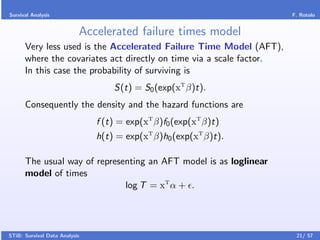
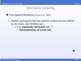
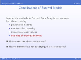
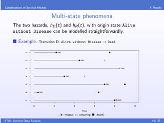
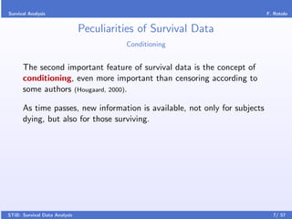
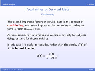
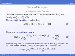
Peculiarities of Survival Data
Censoring
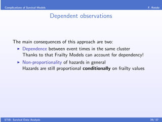
Then the most particular feature of survival data is censoring.
Right censoring (T > t) is very frequent and often unavoidable; all
survival methods account for it.
Interval censoring (T ∈ (l, r ]) is very frequent, too, but much more
ignored in usual practice.
Left censoring (T ≤ t) is very infrequent.
STiB: Survival Data Analysis 6/ 57](https://image.slidesharecdn.com/stibintroductiontosurvivalanalysis-13152948900606-phpapp01-110906024408-phpapp01/85/Introduction-To-Survival-Analysis-11-320.jpg)
![Survival Analysis F. Rotolo
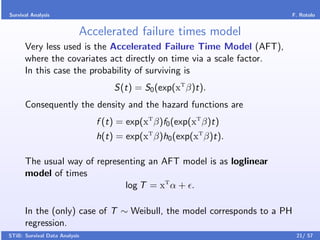
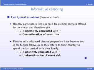
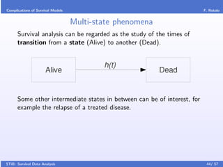
Peculiarities of Survival Data
Censoring
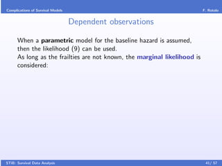
Then the most particular feature of survival data is censoring.
Right censoring (T > t) is very frequent and often unavoidable; all
survival methods account for it.
Interval censoring (T ∈ (l, r ]) is very frequent, too, but much more
ignored in usual practice.
Left censoring (T ≤ t) is very infrequent.
Left truncation is a different concept, concerning the selection
bias introduced by including in the study only subjects having a
survival time greater than a certain value, say t ∗ ; then we do not
observe T but T = T |T > t ∗ .
STiB: Survival Data Analysis 6/ 57](https://image.slidesharecdn.com/stibintroductiontosurvivalanalysis-13152948900606-phpapp01-110906024408-phpapp01/85/Introduction-To-Survival-Analysis-12-320.jpg)


![Survival Analysis F. Rotolo
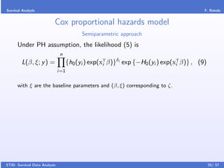
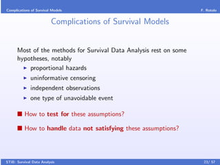
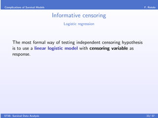
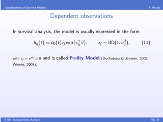
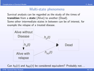
Kaplan–Meier estimator
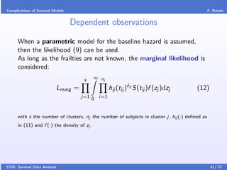
The Kaplan–Meier Product Limit estimator (Kaplan & Meier, 1958)
of the Survival Function is
ˆ Ni ,
SKM (t) = 1− (6)
Ri
i|ti ≤t
with {ti }i the observed event times, Ni the number of events at time ti and Ri the
number of survivors at time ti .
Its variance can be evaluated by the Greenwood’s formula
(Greenwood, 1926; Meier, 1975):
ˆ ˆ Ni
V SKM (t) = [SKM (t)]2 ·
Ri (Ri − Ni )
i|ti ≤t
STiB: Survival Data Analysis 16/ 57](https://image.slidesharecdn.com/stibintroductiontosurvivalanalysis-13152948900606-phpapp01-110906024408-phpapp01/85/Introduction-To-Survival-Analysis-30-320.jpg)