Part of Lecture Series on Automatic Control Systems delivered by me to Final year Diploma in Engg. Students. Easy language and Equally useful for higher level.

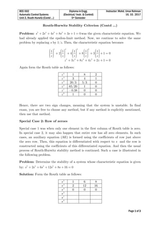
1. BEE-502
Automatic Control Systems
Unit-3, Routh-Hurwitz (Contd ...)
Diploma in Engg.
(Electrical/ Instr. & Control)
5th Semester
Instructor: Mohd. Umar Rehman
16. 10. 2017
Page 1 of 3
Routh-Hurwitz Stability Criterion (Contd ...)
Problem: s ss s s+ + + + + =5 4 3 2
2 4 8 3 1 0 was the given characteristic equation. We
had already applied the epsilon-limit method. Now, we continue to solve the same
problem by replacing s by 1/z. Then, the characteristic equation becomes
z z z z
z z z z
z
z
                + + + + + =               
   
      
+ + + + + =
  
5 4 3 2
5 4 3 2
1 1 1 1
2 4 8 3 1 0
3 8 4 2 1
1
0
Again form the Routh table as follows:
z 5
1 8 2
z 4
3 4 1
z 3
20/3 5/3 0
z 2
65/20 1 0
z 1
−0.38 0 0
z 0
1 0 0
Hence, there are two sign changes, meaning that the system is unstable. In final
exam, you are free to choose any method, but if any method is explicitly mentioned,
then use that method.
Special Case 2: Row of zeroes
Special case 1 was when only one element in the first column of Routh table is zero.
In special case 2, it may also happen that entire row has all zero elements. In such
cases, an auxiliary equation (AE) is formed using the coefficients of row just above
the zero row. Then, this equation is differentiated with respect to s and the row is
constructed using the coefficients of this differentiated equation. And then the usual
process of Routh-Hurwitz stability method is continued. Such a case is illustrated in
the following problem.
Problem: Determine the stability of a system whose characteristic equation is given
by: s s ss s+ + + + + =5 4 3 2
2 6 12 8 16 0
Solution: Form the Routh table as follows:
s 5
1 6 8
s 4
2 12 16
s 3
0 0 0
s 2
s 1
s 0

2. BEE-502
Automatic Control Systems
Unit-3, Routh-Hurwitz (Contd ...)
Diploma in Engg.
(Electrical/ Instr. & Control)
5th Semester
Instructor: Mohd. Umar Rehman
16. 10. 2017
Page 2 of 3
Hence, all the elements of the third row are zero. Now form the auxiliary polynomial
equation using the row just above the zero row as follows:
( )A s ss= + +4 2
6 8
Differentiating w. r. t. s
( )
d
A s s
ds
s= +3
124
Now, replace the zeroes in the third row by the coefficients of above differentiated
equation. Hence, the Routh table modifies to:
s 5
1 6 8
s 4
2 12 16
s 3
4 12 0
s 2
6 16
s 1
1/3 0
s 0
8
There are no sign changes, therefore the system is stable.
Applications of Routh-Hurwitz Criterion
Routh-Hurwitz criterion can be used to determine the range of values of some system
parameter for stability. Let us see one related problem.
Problem: Determine the range of K for stability of a unity feedback control system
whose open-loop transfer function is
( )
( )( )
G s
s s
K
s
=
+ +1 2
Solution: For a unity feedback system, H(s) = 1, the characteristic equation is
given by:
( ) ( )
( )
( )( )
G s H s
G s
K
s s s
s s s K
+ =
+ =
+ =
+ +
+ + =+3 2
1 0
1 0
1
2
2
3
0
1
0
Now, we form the Routh table as follows:

3. BEE-502
Automatic Control Systems
Unit-3, Routh-Hurwitz (Contd ...)
Diploma in Engg.
(Electrical/ Instr. & Control)
5th Semester
Instructor: Mohd. Umar Rehman
16. 10. 2017
Page 3 of 3
s 3
1 2
s 2
3 K
s 1
(6−K)/3
s 0
K
For stability, all the elements in the first column should be positive (no sign change
should be there). So, K > 0 and (6−K)/3 > 0.
⇒K > 0 and K < 6 ⇒ 0 < K < 6. If K = 6, then the system will be marginally
stable and exhibit sustained oscillations.
Assignment Problems
1. For a unity feedback system with the forward transfer function
( )
( )
( )( )
K s
G s
s s s
+
=
+ +
20
2 3
find the range of K to make the system stable.
2. Determine whether the unity feedback system shown in the following figure is
stable
where, ( )
( )( )( )( )
G s
s s s s
=
+ + + +
240
1 2 3 4
*** UNIT-3 ENDS ***