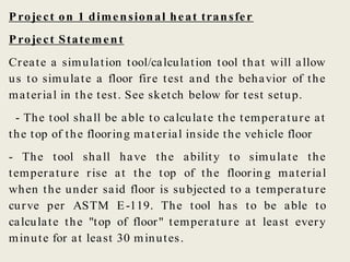
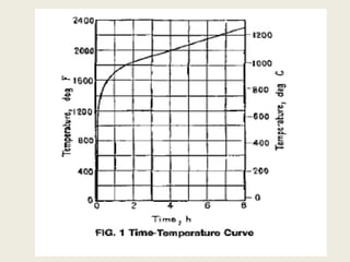
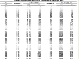
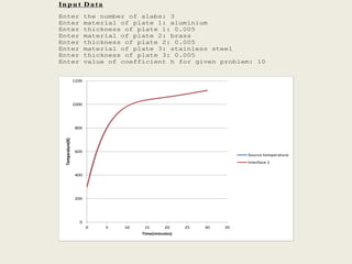
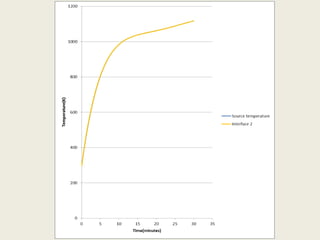
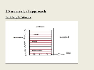
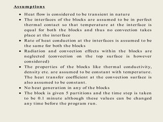
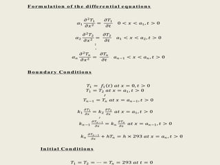
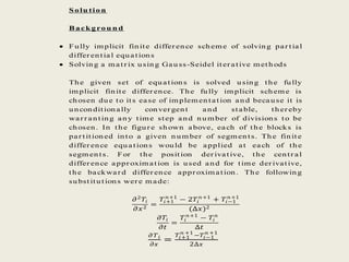
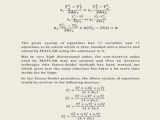
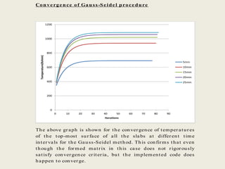
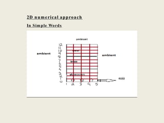
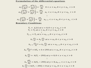
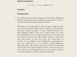
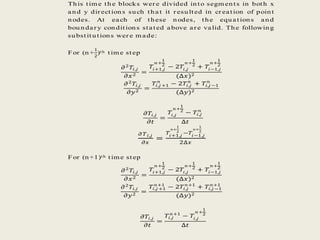
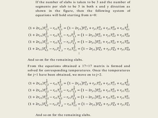
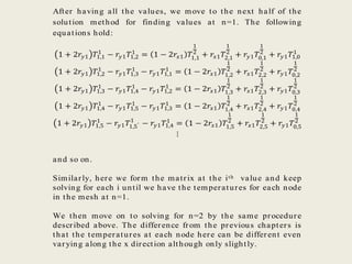
1D and 2D heat transfer project
Project on 1 dimensional heat transfer
Project Statement
Create a simulation tool/calculation tool that will allow
us to simulate a floor fire test and the behavior of the
material in the test. See sketch below for test setup.
- The tool shall be able to calculate the temperature at
the top of the flooring material inside the vehicle floor
- The tool shall have the ability to simulate the
temperature rise at the top of the floorin g material
when the under said floor is subjected to a temperature
curve per ASTM E-119. The tool has to be able to
calculate the "top of floor" temperature at least every
minute for at least 30 minutes.
In pu t Data
Enter the number of slabs: 3
Enter material of plate 1: aluminium
Enter thickness of plate 1: 0.005
Enter material of plate 2: brass
Enter thickness of plate 2: 0.005
Enter material of plate 3: stainless steel
Enter thickness of plate 3: 0.005
Enter value of coefficient h for given problem: 10
0
200
400
600
800
1000
1200
0 5 10 15 20 25 30 35
Temperature(K)
Time(minutes)
Source temperature
Interface 1
Th e gr aph s obtain ed fr om th e pr ogr am h ave been plotted in to
E XCE L an d sh own a bove. Th e gr aph s sh ow th e var iation of
temper atu r e ver su s time at th e differ en t in terfaces. As we can
see, th e tr en d followed is similar to th e sour ce cur ve bu t th e
gr aph s ar e n ot easily distin gu ish a ble. Th e code takes about a
min u te to sh ow u p th e solu tion.
0
200
400
600
800
1000
1200
0 5 10 15 20 25 30 35
Temperature(K)
Time(minutes)
Source temperature
Interface 1
Interface 2
Interface 3
1D numerical approach
In Simple Words
Assu m ption s
 Heat flow is considered to be transient in nature
 The interfaces of the blocks are assumed to be in perfect
thermal contact so th at t emperature at the interface is
equal for both the blocks and thus no convection takes
place at the interface
 Rate of heat conduction at the interfaces is assumed t o be
the same for both the blocks
 Radiation and convection effects within the blocks are
neglected (convection on the top surface is however
considered)
 The properties of the blocks like thermal conductivity,
density etc. are assumed to be constant with temperature.
The heat transfer coefficient at the convection surface is
also assumed to be constan t.
 No heat generation in any of the blocks
 The block is given 5 partitions and the time step is t aken
to be 0.1 minute although these values can be chan ged
any time before the program run.
F o rm u la tion o f th e diffe re n tia l e qu a tio n s
𝛼1
𝜕2 𝑇1
𝜕𝑥2
=
𝜕𝑇1
𝜕𝑡
0 < 𝑥 < 𝑎1, 𝑡 > 0
𝛼2
𝜕2 𝑇2
𝜕𝑥2
=
𝜕𝑇2
𝜕𝑡
𝑎1 < 𝑥 < 𝑎2, 𝑡 > 0
∶
∙
𝛼 𝑛
𝜕2
𝑇𝑛
𝜕𝑥2
=
𝜕𝑇𝑛
𝜕𝑡
𝑎 𝑛−1 < 𝑥 < 𝑎 𝑛 , 𝑡 > 0
B o u n da ry Co n ditio n s
𝑇1 = 𝑓1 𝑡 𝑎𝑡 𝑥 = 0, 𝑡 > 0
𝑇1 = 𝑇2 𝑎𝑡 𝑥 = 𝑎1, 𝑡 > 0
∶
𝑇𝑛−1 = 𝑇𝑛 𝑎𝑡 𝑥 = 𝑎 𝑛−1, 𝑡 > 0
𝑘1
𝜕 𝑇1
𝜕𝑥
= 𝑘2
𝜕 𝑇2
𝜕𝑥
𝑎𝑡 𝑥 = 𝑎1, 𝑡 > 0
∶
𝑘 𝑛−1
𝜕 𝑇 𝑛 −1
𝜕𝑥
= 𝑘 𝑛
𝜕 𝑇 𝑛
𝜕𝑥
𝑎𝑡 𝑥 = 𝑎 𝑛−1, 𝑡 > 0
𝑘 𝑛
𝜕 𝑇 𝑛 −1
𝜕𝑥
+ ℎ𝑇𝑛 = ℎ × 293 𝑎𝑡 𝑥 = 𝑎 𝑛 , 𝑡 > 0
In itia l Co n ditio n s
𝑇1 = 𝑇2 = ⋯ = 𝑇𝑛 = 293 𝑎𝑡 𝑡 = 0
Solu tion
Backgrou n d
 Fully implicit finite differ ence scheme of solving par tial
differ ential equations
 Solving a matr ix using Gau ss-Seidel iter ative methods
The given set of equations is solved using the fully
implicit finite differ ence. The fully implicit scheme is
chosen due to its ease of implementation and because it is
unconditionally conver gent and stable, ther eby
war r anting any time step and number of divisions to be
chosen. In the figur e shown above, each of the blocks is
par titioned into a given n umber of segments. The finite
differ ence equations would be applied at each of the
segments. For the position der ivative, the centr al
differ ence appr oximation is used and for time der ivative,
the backwar d differ ence appr oximation. The following
substitutions wer e m ade:
𝜕2
𝑇𝑖
𝜕𝑥2
=
𝑇𝑖+1
𝑛+1
− 2𝑇𝑖
𝑛+1
+ 𝑇𝑖−1
𝑛+1
(∆𝑥)2
𝜕𝑇𝑖
𝜕𝑡
=
𝑇𝑖
𝑛+1
− 𝑇𝑖
𝑛
∆𝑡
𝜕 𝑇 𝑖
𝜕𝑥
=
𝑇𝑖+1
𝑛 +1
−𝑇𝑖−1
𝑛 +1
2∆𝑥
If t h e nu m ber of slabs is t aken t o be 3 an d t h e n u m ber of
n odes per slab t o be 5 as sh own in t h e figu r e, t h en t h e
followin g syst em of equ at ion s will h old st ar t in g fr om n =0:
1 + 2𝑟1 𝑇1
1
− 𝑟1 𝑇2
1
= 𝑇1
0
+ 𝑟1 𝑇0
1
1 + 2𝑟1 𝑇2
1
− 𝑟1 𝑇1
1
− 𝑟1 𝑇3
1
= 𝑇2
0
1 + 2𝑟1 𝑇3
1
− 𝑟1 𝑇2
1
− 𝑟1 𝑇4
1
= 𝑇3
0
1 + 2𝑟1 𝑇4
1
− 𝑟1 𝑇3
1
− 𝑟1 𝑇4′
1
= 𝑇4
0
An im agin ar y n ode 𝑇4′
1
is t aken h er e t o sat isfy t h e
con dit ion s. Sim ilar ly, ot h er su ch n odes will be t aken wh en
r equ ir ed t o for m t h e given m at r ix alt h ou gh t h e valu es
obt ain ed for t h ese var iables will h old n o m ean in g.
Con t in u in g wit h t h e syst em of equ at ion s:
1 + 2𝑟2 𝑇4
1
− 𝑟2 𝑇4′′
1
− 𝑟2 𝑇5
1
= 𝑇4
0
1 + 2𝑟2 𝑇5
1
− 𝑟2 𝑇4
1
− 𝑟2 𝑇6
1
= 𝑇5
0
1 + 2𝑟2 𝑇6
1
− 𝑟2 𝑇5
1
− 𝑟2 𝑇7
1
= 𝑇6
0
1 + 2𝑟2 𝑇7
1
− 𝑟2 𝑇6
1
− 𝑟2 𝑇8
1
= 𝑇7
0
1 + 2𝑟2 𝑇8
1
− 𝑟2 𝑇7
1
− 𝑟2 𝑇8′
1
= 𝑇8
0
1 + 2𝑟3 𝑇8
1
− 𝑟3 𝑇8′′
1
− 𝑟3 𝑇9
1
= 𝑇8
0
1 + 2𝑟3 𝑇9
1
− 𝑟3 𝑇8
1
− 𝑟3 𝑇10
1
= 𝑇9
0
1 + 2𝑟3 𝑇10
1
− 𝑟3 𝑇9
1
− 𝑟3 𝑇11
1
= 𝑇10
0
1 + 2𝑟3 𝑇11
1
− 𝑟3 𝑇10
1
− 𝑟3 𝑇12
1
= 𝑇11
0
1 + 2𝑟3 𝑇12
1
− 𝑟3 𝑇11
1
− 𝑟3 𝑇12′
1
= 𝑇12
0
𝑘1
𝑇
4′
1
− 𝑇3
1
2∆𝑥1
= 𝑘2
𝑇5
1
− 𝑇
4′′
1
2∆𝑥2
𝑘2
𝑇
8′
1
−𝑇7
1
2∆𝑥2
= 𝑘3
𝑇9
1
−𝑇
8′′
1
2∆𝑥3
𝑘3
𝑇12′
1
− 𝑇11
1
2∆𝑥3
+ ℎ 𝑇12
1
− 293 = 0
Th e given syst em of equ at ion s h as 17 var iables an d 17
equ at ion s t o be solved wh ich is t h en en coded in t o a m at r ix an d
solved by MATLAB u sin g t h e com m an d A b.
Bu t in ver y h igh dim en sion al codes, t h e n on -it er at ive codes
u sed by MATLAB m ay n ot su cceed an d t h u s an it er at ive
t ech n iqu e (t h e Gau ss-Seidel m et h od) h as been wor ked ou t
wh ich gives ju st t h e sam e solu t ion s bu t t akes a lot m or e t im e
in side t h e for loops.
In t h e Gau ss-Seidel pr ocedu r e, t h e above syst em of equ at ion s
wou ld be wr it t en in t h e followin g m an n er :
𝑇1
1
=
𝑇1
0
+ 𝑟1 𝑇0
1
+ 𝑟1 𝑇2
1
1 + 2𝑟1
𝑇2
1
=
𝑇2
0
+ 𝑟1 𝑇1
1
+ 𝑟1 𝑇3
1
1 + 2𝑟1
𝑇3
1
=
𝑇3
0
+ 𝑟1 𝑇2
1
+ 𝑟1 𝑇4
1
1 + 2𝑟1
𝑇4
1
=
𝑇4
0
+ 𝑟1 𝑇3
1
+ 𝑟1 𝑇4′
1
1 + 2𝑟1
𝑇4′
1
=
−𝑇4
0
− 𝑟2 𝑇3
1
+ (1 + 2𝑟2)𝑇4
1
𝑟2
𝑇5
1
=
𝑇5
0
+𝑟2 𝑇6
1+𝑟2 𝑇4
1
1+2𝑟2
and so on till each node is explicitly written in terms of other
nodes. A set of values for all 17 nodes is then assumed and the
1st node is then calculated from the above equation. The
modified 1st node and the remaining nodes are then put into
the 2nd node equation. The procedure keeps repeating till the
consecutive values of the same node converge. For the Gauss -
Seidel method, this convergence mostly happens if the given
matrix is tri-diagonal or diagonally dominant. In this case,
even though the formed matrix is neither, it is very close to
being a tri-diagonal matrix and thus the solution does
converge.
After the 17 values for n=0 are obtained either by direct matrix
solutions or iterative procedures, the matrix is solved again for
n=1 and so on till all required values for all times are not
obtained.
The code for the above solution has however been developed for
any number of slabs and partitions in MATLAB. The code
developed is printed in Appendix B.
In pu t D a ta
Enter the number of slabs: 3
Enter material of plate 1: aluminium
Enter thickness of plate 1: 0.005
Enter material of plate 2: brass
Enter thickness of plate 2: 0.005
Enter material of plate 3: stainless steel
Enter thickness of plate 3: 0.005
Enter value of coefficent h for given problem: 10
With o u t Ga u s s -Se ide l ite ra tio n
0
200
400
600
800
1000
1200
0 5 10 15 20 25 30 35
Temperature(K)
Time(minutes)
Source temperature
Interface 1
Interface 2
Interface 3
With Ga u ss -Se ide l ite ra tio n
0
200
400
600
800
1000
1200
0 5 10 15 20 25 30 35
Temperature(K)
Time(minutes)
Source temperature
Interface 1 gs
Interface 2 gs
Interface 3 gs
Com parison (w ith an d w ith ou t Gau ss -Se ide l)
As we can see, both th e non -iter ative and the iter ative
pr ogr ams yield exactly the same r esults with the respective
gr aphs in both the methods over lapping. The iter ative
pr ocedur e however takes up slightly mor e time and memor y
space although it guar antees solution for ver y lar ge matr ices
too.
0
200
400
600
800
1000
1200
0 5 10 15 20 25 30 35
Temperature(K)
Time(minutes)
Source temperature
Interface 1 gs
Interface 2 gs
Interface 3 gs
Interface 1
Interface 2
Interface 3
Con ve rge n ce of Gau ss-Se ide l proce du re
The above graph is shown for the convergence of temperatures
of the top-most surface of all the slabs at different time
intervals for the Gauss-Seidel method. This confirms that even
though the formed matrix in this case does not rigorously
satisfy convergence criteria, but the implemented code does
happen to converge.
0
200
400
600
800
1000
1200
0 10 20 30 40 50 60 70 80 90
Temperature(Kelvin)
Iterations
5min
10min
15min
20min
25min
Improvements
 converting the program into GUI
 increasing options for user to input values like
surrounding temperature etc.
 creating separate functions for some part of the code for
better reusability and optimizing code to work faster
 validating the answer obtained through experimental
techniques
 making the problem more and more generalized by
reducing number of assumptions
Conclusion
The fully implicit finite difference method, both by with and
without Gauss-Seidel iteration, gives a seemingly good and
accurate solution which can now be verified by experimental
techniques. Now that a seemingly right methodology has been
accomplished, the scope of expanding the project to higher
dimensions (2D has been included next) or including radiation
conditions always remains.
2D numerical approach
In Simple Words
Assumptions
 Heat flow is considered to be transient in nature
 The interfaces of the blocks are assumed to be in perfect
thermal contact so that temperature at the interface is
equal for both the blocks and thus no convection takes
place at the interface.
 Rate of heat conduction at the interfaces is assumed to be
the same for both the blocks
 Radiation and convection effects within the blocks are
neglected (convection on the top surface and the sides is
however considered)
 The properties of the blocks like thermal conductivity,
density etc. are assumed to be constant with temperature.
The heat transfer coefficient at the convection surface is
also assumed to be constant.
 No heat generation in any of the blocks
 There are two values of interface temperatures fou nd at
each time step which differ by a slight proportion. Thus,
the first has been taken as the valid temperature in such
a scenario.
F orm u lation of th e diffe re n tial e qu ation s
𝛼1
𝜕2
𝑇1
𝜕𝑥2
+
𝜕2
𝑇1
𝜕𝑦2
=
𝜕𝑇1
𝜕𝑡
0 < 𝑥 < 𝑎1, 0 < 𝑦 < 𝑎 𝑦, 𝑡 > 0
𝛼2
𝜕2
𝑇2
𝜕𝑥2
+
𝜕2
𝑇2
𝜕𝑦2
=
𝜕𝑇2
𝜕𝑡
𝑎1 < 𝑥 < 𝑎2, 0 < 𝑦 < 𝑎 𝑦, 𝑡 > 0
⋮
𝛼 𝑛
𝜕2 𝑇𝑛
𝜕𝑥2
+
𝜕2 𝑇𝑛
𝜕𝑦2
=
𝜕𝑇𝑛
𝜕𝑡
𝑎 𝑛−1 < 𝑥 < 𝑎 𝑛 , 0 < 𝑦 < 𝑎 𝑦, 𝑡 > 0
Bou n dary Con dition s
𝑇1 = 𝑓1 𝑡 𝑎𝑡 𝑥 = 0, 0 < 𝑦 < 𝑎 𝑦 , 𝑡 > 0
𝑇1 = 𝑇2 𝑎𝑡 𝑥 = 𝑎1, 0 < 𝑦 < 𝑎 𝑦 , 𝑡 > 0
∶
𝑇𝑛−1 = 𝑇𝑛 𝑎𝑡 𝑥 = 𝑎 𝑛−1, 0 < 𝑦 < 𝑎 𝑦 , 𝑡 > 0
𝑘1
𝜕 𝑇1
𝜕𝑥
= 𝑘2
𝜕 𝑇2
𝜕𝑥
𝑎𝑡 𝑥 = 𝑎1, 0 < 𝑦 < 𝑎 𝑦 , 𝑡 > 0
∶
𝑘 𝑛−1
𝜕 𝑇 𝑛 −1
𝜕𝑥
= 𝑘 𝑛
𝜕 𝑇 𝑛
𝜕𝑥
𝑎𝑡 𝑥 = 𝑎 𝑛−1, 0 < 𝑦 < 𝑎 𝑦 , 𝑡 > 0
𝑘 𝑛
𝜕 𝑇 𝑛 −1
𝜕𝑥
+ ℎ𝑇𝑛 = ℎ × 293 𝑎𝑡 𝑥 = 𝑎 𝑛 , 0 < 𝑦 < 𝑎 𝑦 , 𝑡 > 0
𝑘1
𝜕 𝑇1
𝜕𝑦
= ℎ(𝑇1 − 293) 𝑎𝑡 𝑦 = 0, 0 < 𝑥 < 𝑎1 𝑡 > 0
⋮
𝑘 𝑛
𝜕𝑇𝑛
𝜕𝑦
= ℎ(𝑇𝑛 − 293) 𝑎𝑡 𝑦 = 0, 𝑎 𝑛−1 < 𝑥 < 𝑎 𝑛 𝑡 > 0
𝑘1
𝜕 𝑇1
𝜕𝑦
+ ℎ(𝑇1 − 293) = 0 𝑎𝑡 𝑦 = 𝑎 𝑦 , 0 < 𝑥 < 𝑎1 𝑡 > 0
Initial Conditions
𝑇1 = 𝑇2 = ⋯ = 𝑇𝑛 = 293 𝑎𝑡 𝑡 = 0
Solution
Background
 The alternating direction implicit (ADI) finite difference
scheme of solving partial differential equations which is
well suited for a 2D heat transfer problem
The above set of equations is solved using a slight variant
of the fully implicit FDM scheme called the alternating
direction implicit method. A usual implementation of a
fully implicit FDM in this case would result in a near
penta-diagonal matrix which would have to be coded all
over again. Instead, the ADI scheme breaks a time step
into two halves. In the first half, the x-derivative is
written as an implicit central-difference approximation
and the y-derivative as an explicit central-difference
approximation. The reverse holds true for the second half
of the time step. Each of these halves result in matrices
very similar to tri-diagonal matrix, the results of which
are then combined to obtain the final solution.
This time the blocks wer e divided into segments in both x
and y dir ections such tha t it r esulted in cr eation of point
nodes. At each of these nodes, the equations and
boundar y conditions stated above ar e valid. The following
substitutions wer e m ade:
For (n+
1
2
)t h time step
𝜕2 𝑇𝑖,𝑗
𝜕𝑥2
=
𝑇𝑖+1,𝑗
𝑛+
1
2
− 2𝑇𝑖,𝑗
𝑛+
1
2
+ 𝑇𝑖−1,𝑗
𝑛+
1
2
(∆𝑥)2
𝜕2 𝑇𝑖,𝑗
𝜕𝑦2
=
𝑇𝑖,𝑗 +1
𝑛
− 2𝑇𝑖,𝑗
𝑛
+ 𝑇𝑖,𝑗 −1
𝑛
(∆𝑦)2
𝜕𝑇𝑖,𝑗
𝜕𝑡
=
𝑇𝑖,𝑗
𝑛+
1
2
− 𝑇𝑖,𝑗
𝑛
∆𝑡
𝜕 𝑇 𝑖,𝑗
𝜕𝑥
=
𝑇𝑖+1,𝑗
𝑛+
1
2
−𝑇𝑖−1,𝑗
𝑛+
1
2
2∆𝑥
For (n+1)t h time step
𝜕2 𝑇𝑖,𝑗
𝜕𝑥2
=
𝑇𝑖+1,𝑗
𝑛+
1
2
− 2𝑇𝑖,𝑗
𝑛+
1
2
+ 𝑇𝑖−1,𝑗
𝑛+
1
2
(∆𝑥)2
𝜕2
𝑇𝑖,𝑗
𝜕𝑦2
=
𝑇𝑖,𝑗 +1
𝑛+1
− 2𝑇𝑖,𝑗
𝑛+1
+ 𝑇𝑖,𝑗 −1
𝑛+1
(∆𝑦)2
𝜕𝑇𝑖,𝑗
𝜕𝑡
=
𝑇𝑖,𝑗
𝑛+1
− 𝑇𝑖,𝑗
𝑛+
1
2
∆𝑡
If the number of slabs is taken to be 3 and the number of
segments per slab to be 5 in both x and y direction as
shown in the figure, then the following system of
equations will hold starting from n=0:
1 + 2𝑟𝑥1 𝑇1,1
1
2
− 𝑟𝑥1 𝑇2,1
1
2
= 1 − 2𝑟𝑦1 𝑇1,1
0
+ 𝑟𝑦1 𝑇1,2
0
+ 𝑟𝑦1 𝑇1,0
0
+ 𝑟𝑥1 𝑇0,1
1
2
1 + 2𝑟𝑥1 𝑇2,1
1
2
− 𝑟𝑥1 𝑇3,1
1
2
− 𝑟𝑥1 𝑇1,1
1
2
= 1 − 2𝑟𝑦1 𝑇2,1
0
+ 𝑟𝑦1 𝑇2,2
0
+ 𝑟𝑦1 𝑇2,0
0
1 + 2𝑟𝑥1 𝑇3,1
1
2
− 𝑟𝑥1 𝑇4,1
1
2
− 𝑟𝑥1 𝑇2,1
1
2
= 1 − 2𝑟𝑦1 𝑇3,1
0
+ 𝑟𝑦1 𝑇3,2
0
+ 𝑟𝑦1 𝑇3,0
0
1 + 2𝑟𝑥1 𝑇4,1
1
2
− 𝑟𝑥1 𝑇4′ ,1
1
2
− 𝑟𝑥1 𝑇3,1
1
2
= 1 − 2𝑟𝑦1 𝑇4,1
0
+ 𝑟𝑦1 𝑇4,2
0
+ 𝑟𝑦1 𝑇4,0
0
⋮
And so on for the remaining slabs.
From the equations obtained a 17×17 matrix is formed and
solved for corresponding temperatures. Once the temperatures
for j=1 have been obtained, we move on to j=2.
1 + 2𝑟𝑥1 𝑇1,2
1
2
− 𝑟𝑥1 𝑇2,2
1
2
= 1 − 2𝑟𝑦1 𝑇1,2
0
+ 𝑟𝑦1 𝑇1,3
0
+ 𝑟𝑦1 𝑇1,1
0
+ 𝑟𝑥1 𝑇0,2
1
2
1 + 2𝑟𝑥1 𝑇2,2
1
2
− 𝑟𝑥1 𝑇3,2
1
2
− 𝑟𝑥1 𝑇1,2
1
2
= 1 − 2𝑟𝑦1 𝑇2,2
0
+ 𝑟𝑦1 𝑇2,3
0
+ 𝑟𝑦1 𝑇2,1
0
1 + 2𝑟𝑥1 𝑇3,2
1
2
− 𝑟𝑥1 𝑇4,2
1
2
− 𝑟𝑥1 𝑇2,2
1
2
= 1 − 2𝑟𝑦1 𝑇3,2
0
+ 𝑟𝑦1 𝑇3,3
0
+ 𝑟𝑦1 𝑇3,1
0
1 + 2𝑟𝑥1 𝑇4,2
1
2
− 𝑟𝑥1 𝑇4′ ,2
1
2
− 𝑟𝑥1 𝑇3,2
1
2
= 1 − 2𝑟𝑦1 𝑇4,2
0
+ 𝑟𝑦1 𝑇4,3
0
+ 𝑟𝑦1 𝑇4,1
0
⋮
And so on for the remaining slabs.
After having all the values, we move to the next half of the
solution method for finding values at n=1. The following
equations hold:
1 + 2𝑟𝑦1 𝑇1,1
1
− 𝑟𝑦1 𝑇1,2
1
= 1 − 2𝑟𝑥1 𝑇1,1
1
2
+ 𝑟𝑥1 𝑇2,1
1
2
+ 𝑟𝑦1 𝑇0,1
1
2
+ 𝑟𝑦1 𝑇1,0
1
1 + 2𝑟𝑦1 𝑇1,2
1
− 𝑟𝑦1 𝑇1,3
1
− 𝑟𝑦1 𝑇1,1
1
= 1 − 2𝑟𝑥1 𝑇1,2
1
2
+ 𝑟𝑥1 𝑇2,2
1
2
+ 𝑟𝑦1 𝑇0,2
1
2
1 + 2𝑟𝑦1 𝑇1,3
1
− 𝑟𝑦1 𝑇1,4
1
− 𝑟𝑦1 𝑇1,2
1
= 1 − 2𝑟𝑥1 𝑇1,3
1
2
+ 𝑟𝑥1 𝑇2,3
1
2
+ 𝑟𝑦1 𝑇0,3
1
2
1 + 2𝑟𝑦1 𝑇1,4
1
− 𝑟𝑦1 𝑇1,5
1
− 𝑟𝑦1 𝑇1,3
1
= 1 − 2𝑟𝑥1 𝑇1,4
1
2
+ 𝑟𝑥1 𝑇2,4
1
2
+ 𝑟𝑦1 𝑇0,4
1
2
1 + 2𝑟𝑦1 𝑇1,5
1
− 𝑟𝑦1 𝑇1,5′
1
− 𝑟𝑦1 𝑇1,4
1
= 1 − 2𝑟𝑥1 𝑇1,5
1
2
+ 𝑟𝑥1 𝑇2,5
1
2
+ 𝑟𝑦1 𝑇0,5
1
2
⋮
and so on.
Similarly, here we form the matrix at the ith value and keep
solving for each i until we have the temperatures for each node
in the mesh at n=1.
We then move on to solving for n=2 by the same procedure
described above. The difference from the previous chapters is
that the temperatures at each node here can be different even
varying along the x direction although only slightly.
In pu t Data
Enter the number of slabs: 3
Enter material of plate 1: aluminium
Enter thickness of plate 1: 0.005
Enter material of plate 2: brass
Enter thickness of plate 2: 0.005
Enter material of plate 3: stainless steel
Enter thickness of plate 3: 0.005
Enter equal width of all plates: 0.01
Enter value of coefficent h for given problem: 10
The gr aph above has been shown for the cor ner nodes of all the
inter faces and follows similar tr ends as discussed in the
pr evious chapter s.
0
200
400
600
800
1000
1200
0 5 10 15 20 25 30 35
Temperature(K)
Time(minutes)
node 1
node 2
node 3
Source temperature
The graph above shows temperature curves for all nodes of the
top surface. As we see, the temperature variation along the y
direction is not much and the temperature curves for all these
nodes overlap.
0
200
400
600
800
1000
1200
0 5 10 15 20 25 30 35
Temperature(K)
Time(minutes)
Top Surface
Source temperature
node 1
node 2
node 3
node 4
node 5
This graph shows the temperature variation along the top
surface at time t=30 min. As expected, the temperature is
symmetric with respect to the middle node with heat flowing
from both sides of the middle node to the surroundings at
ambient temperature.
1092.2
1092.4
1092.6
1092.8
1093
1093.2
1093.4
1093.6
1093.8
0 1 2 3 4 5 6
Temperature(K)
node
Top Surface
30 min
Improvements
 converting the program into GUI
 increasing options for user to input values like
surrounding temperature etc.
 creating separate functions for some part of the code for
better reusability and optimizing code to work faster
 validating the answer obtained through experimental
techniques
 making the problem more and more generalized by
reducing number of assumptions
 can be extended to the 3 dimensional case
Conclusion
The ADI finite difference technique works for the 2
dimensional case and gives good results which can now be
validated using experimental techniques.
References
 Heat conduction by M Necati Ozisik
 http://highered.mcgraw-hill.com/sites/dl/free/0073129305/314124/cen29305_ch04.pdf
 en.wikepedia.org
 www.mathworks.in
 www.wolframalpha.org
 Computational Fluid Dynamics by John D. Anderson
Thank You!!!

project presentation

  • 1.
    1D and 2Dheat transfer project
  • 2.
    Project on 1dimensional heat transfer Project Statement Create a simulation tool/calculation tool that will allow us to simulate a floor fire test and the behavior of the material in the test. See sketch below for test setup. - The tool shall be able to calculate the temperature at the top of the flooring material inside the vehicle floor - The tool shall have the ability to simulate the temperature rise at the top of the floorin g material when the under said floor is subjected to a temperature curve per ASTM E-119. The tool has to be able to calculate the "top of floor" temperature at least every minute for at least 30 minutes.
  • 5.
    In pu tData Enter the number of slabs: 3 Enter material of plate 1: aluminium Enter thickness of plate 1: 0.005 Enter material of plate 2: brass Enter thickness of plate 2: 0.005 Enter material of plate 3: stainless steel Enter thickness of plate 3: 0.005 Enter value of coefficient h for given problem: 10 0 200 400 600 800 1000 1200 0 5 10 15 20 25 30 35 Temperature(K) Time(minutes) Source temperature Interface 1
  • 7.
    Th e graph s obtain ed fr om th e pr ogr am h ave been plotted in to E XCE L an d sh own a bove. Th e gr aph s sh ow th e var iation of temper atu r e ver su s time at th e differ en t in terfaces. As we can see, th e tr en d followed is similar to th e sour ce cur ve bu t th e gr aph s ar e n ot easily distin gu ish a ble. Th e code takes about a min u te to sh ow u p th e solu tion. 0 200 400 600 800 1000 1200 0 5 10 15 20 25 30 35 Temperature(K) Time(minutes) Source temperature Interface 1 Interface 2 Interface 3
  • 8.
  • 9.
    Assu m ptions  Heat flow is considered to be transient in nature  The interfaces of the blocks are assumed to be in perfect thermal contact so th at t emperature at the interface is equal for both the blocks and thus no convection takes place at the interface  Rate of heat conduction at the interfaces is assumed t o be the same for both the blocks  Radiation and convection effects within the blocks are neglected (convection on the top surface is however considered)  The properties of the blocks like thermal conductivity, density etc. are assumed to be constant with temperature. The heat transfer coefficient at the convection surface is also assumed to be constan t.  No heat generation in any of the blocks  The block is given 5 partitions and the time step is t aken to be 0.1 minute although these values can be chan ged any time before the program run.
  • 10.
    F o rmu la tion o f th e diffe re n tia l e qu a tio n s 𝛼1 𝜕2 𝑇1 𝜕𝑥2 = 𝜕𝑇1 𝜕𝑡 0 < 𝑥 < 𝑎1, 𝑡 > 0 𝛼2 𝜕2 𝑇2 𝜕𝑥2 = 𝜕𝑇2 𝜕𝑡 𝑎1 < 𝑥 < 𝑎2, 𝑡 > 0 ∶ ∙ 𝛼 𝑛 𝜕2 𝑇𝑛 𝜕𝑥2 = 𝜕𝑇𝑛 𝜕𝑡 𝑎 𝑛−1 < 𝑥 < 𝑎 𝑛 , 𝑡 > 0 B o u n da ry Co n ditio n s 𝑇1 = 𝑓1 𝑡 𝑎𝑡 𝑥 = 0, 𝑡 > 0 𝑇1 = 𝑇2 𝑎𝑡 𝑥 = 𝑎1, 𝑡 > 0 ∶ 𝑇𝑛−1 = 𝑇𝑛 𝑎𝑡 𝑥 = 𝑎 𝑛−1, 𝑡 > 0 𝑘1 𝜕 𝑇1 𝜕𝑥 = 𝑘2 𝜕 𝑇2 𝜕𝑥 𝑎𝑡 𝑥 = 𝑎1, 𝑡 > 0 ∶ 𝑘 𝑛−1 𝜕 𝑇 𝑛 −1 𝜕𝑥 = 𝑘 𝑛 𝜕 𝑇 𝑛 𝜕𝑥 𝑎𝑡 𝑥 = 𝑎 𝑛−1, 𝑡 > 0 𝑘 𝑛 𝜕 𝑇 𝑛 −1 𝜕𝑥 + ℎ𝑇𝑛 = ℎ × 293 𝑎𝑡 𝑥 = 𝑎 𝑛 , 𝑡 > 0 In itia l Co n ditio n s 𝑇1 = 𝑇2 = ⋯ = 𝑇𝑛 = 293 𝑎𝑡 𝑡 = 0
  • 11.
    Solu tion Backgrou nd  Fully implicit finite differ ence scheme of solving par tial differ ential equations  Solving a matr ix using Gau ss-Seidel iter ative methods The given set of equations is solved using the fully implicit finite differ ence. The fully implicit scheme is chosen due to its ease of implementation and because it is unconditionally conver gent and stable, ther eby war r anting any time step and number of divisions to be chosen. In the figur e shown above, each of the blocks is par titioned into a given n umber of segments. The finite differ ence equations would be applied at each of the segments. For the position der ivative, the centr al differ ence appr oximation is used and for time der ivative, the backwar d differ ence appr oximation. The following substitutions wer e m ade: 𝜕2 𝑇𝑖 𝜕𝑥2 = 𝑇𝑖+1 𝑛+1 − 2𝑇𝑖 𝑛+1 + 𝑇𝑖−1 𝑛+1 (∆𝑥)2 𝜕𝑇𝑖 𝜕𝑡 = 𝑇𝑖 𝑛+1 − 𝑇𝑖 𝑛 ∆𝑡 𝜕 𝑇 𝑖 𝜕𝑥 = 𝑇𝑖+1 𝑛 +1 −𝑇𝑖−1 𝑛 +1 2∆𝑥
  • 12.
    If t he nu m ber of slabs is t aken t o be 3 an d t h e n u m ber of n odes per slab t o be 5 as sh own in t h e figu r e, t h en t h e followin g syst em of equ at ion s will h old st ar t in g fr om n =0: 1 + 2𝑟1 𝑇1 1 − 𝑟1 𝑇2 1 = 𝑇1 0 + 𝑟1 𝑇0 1 1 + 2𝑟1 𝑇2 1 − 𝑟1 𝑇1 1 − 𝑟1 𝑇3 1 = 𝑇2 0 1 + 2𝑟1 𝑇3 1 − 𝑟1 𝑇2 1 − 𝑟1 𝑇4 1 = 𝑇3 0 1 + 2𝑟1 𝑇4 1 − 𝑟1 𝑇3 1 − 𝑟1 𝑇4′ 1 = 𝑇4 0 An im agin ar y n ode 𝑇4′ 1 is t aken h er e t o sat isfy t h e con dit ion s. Sim ilar ly, ot h er su ch n odes will be t aken wh en r equ ir ed t o for m t h e given m at r ix alt h ou gh t h e valu es obt ain ed for t h ese var iables will h old n o m ean in g. Con t in u in g wit h t h e syst em of equ at ion s: 1 + 2𝑟2 𝑇4 1 − 𝑟2 𝑇4′′ 1 − 𝑟2 𝑇5 1 = 𝑇4 0 1 + 2𝑟2 𝑇5 1 − 𝑟2 𝑇4 1 − 𝑟2 𝑇6 1 = 𝑇5 0 1 + 2𝑟2 𝑇6 1 − 𝑟2 𝑇5 1 − 𝑟2 𝑇7 1 = 𝑇6 0 1 + 2𝑟2 𝑇7 1 − 𝑟2 𝑇6 1 − 𝑟2 𝑇8 1 = 𝑇7 0 1 + 2𝑟2 𝑇8 1 − 𝑟2 𝑇7 1 − 𝑟2 𝑇8′ 1 = 𝑇8 0 1 + 2𝑟3 𝑇8 1 − 𝑟3 𝑇8′′ 1 − 𝑟3 𝑇9 1 = 𝑇8 0 1 + 2𝑟3 𝑇9 1 − 𝑟3 𝑇8 1 − 𝑟3 𝑇10 1 = 𝑇9 0 1 + 2𝑟3 𝑇10 1 − 𝑟3 𝑇9 1 − 𝑟3 𝑇11 1 = 𝑇10 0 1 + 2𝑟3 𝑇11 1 − 𝑟3 𝑇10 1 − 𝑟3 𝑇12 1 = 𝑇11 0 1 + 2𝑟3 𝑇12 1 − 𝑟3 𝑇11 1 − 𝑟3 𝑇12′ 1 = 𝑇12 0
  • 13.
    𝑘1 𝑇 4′ 1 − 𝑇3 1 2∆𝑥1 = 𝑘2 𝑇5 1 −𝑇 4′′ 1 2∆𝑥2 𝑘2 𝑇 8′ 1 −𝑇7 1 2∆𝑥2 = 𝑘3 𝑇9 1 −𝑇 8′′ 1 2∆𝑥3 𝑘3 𝑇12′ 1 − 𝑇11 1 2∆𝑥3 + ℎ 𝑇12 1 − 293 = 0 Th e given syst em of equ at ion s h as 17 var iables an d 17 equ at ion s t o be solved wh ich is t h en en coded in t o a m at r ix an d solved by MATLAB u sin g t h e com m an d A b. Bu t in ver y h igh dim en sion al codes, t h e n on -it er at ive codes u sed by MATLAB m ay n ot su cceed an d t h u s an it er at ive t ech n iqu e (t h e Gau ss-Seidel m et h od) h as been wor ked ou t wh ich gives ju st t h e sam e solu t ion s bu t t akes a lot m or e t im e in side t h e for loops. In t h e Gau ss-Seidel pr ocedu r e, t h e above syst em of equ at ion s wou ld be wr it t en in t h e followin g m an n er : 𝑇1 1 = 𝑇1 0 + 𝑟1 𝑇0 1 + 𝑟1 𝑇2 1 1 + 2𝑟1 𝑇2 1 = 𝑇2 0 + 𝑟1 𝑇1 1 + 𝑟1 𝑇3 1 1 + 2𝑟1 𝑇3 1 = 𝑇3 0 + 𝑟1 𝑇2 1 + 𝑟1 𝑇4 1 1 + 2𝑟1 𝑇4 1 = 𝑇4 0 + 𝑟1 𝑇3 1 + 𝑟1 𝑇4′ 1 1 + 2𝑟1
  • 14.
    𝑇4′ 1 = −𝑇4 0 − 𝑟2 𝑇3 1 +(1 + 2𝑟2)𝑇4 1 𝑟2 𝑇5 1 = 𝑇5 0 +𝑟2 𝑇6 1+𝑟2 𝑇4 1 1+2𝑟2 and so on till each node is explicitly written in terms of other nodes. A set of values for all 17 nodes is then assumed and the 1st node is then calculated from the above equation. The modified 1st node and the remaining nodes are then put into the 2nd node equation. The procedure keeps repeating till the consecutive values of the same node converge. For the Gauss - Seidel method, this convergence mostly happens if the given matrix is tri-diagonal or diagonally dominant. In this case, even though the formed matrix is neither, it is very close to being a tri-diagonal matrix and thus the solution does converge. After the 17 values for n=0 are obtained either by direct matrix solutions or iterative procedures, the matrix is solved again for n=1 and so on till all required values for all times are not obtained. The code for the above solution has however been developed for any number of slabs and partitions in MATLAB. The code developed is printed in Appendix B.
  • 15.
    In pu tD a ta Enter the number of slabs: 3 Enter material of plate 1: aluminium Enter thickness of plate 1: 0.005 Enter material of plate 2: brass Enter thickness of plate 2: 0.005 Enter material of plate 3: stainless steel Enter thickness of plate 3: 0.005 Enter value of coefficent h for given problem: 10 With o u t Ga u s s -Se ide l ite ra tio n 0 200 400 600 800 1000 1200 0 5 10 15 20 25 30 35 Temperature(K) Time(minutes) Source temperature Interface 1 Interface 2 Interface 3
  • 16.
    With Ga uss -Se ide l ite ra tio n 0 200 400 600 800 1000 1200 0 5 10 15 20 25 30 35 Temperature(K) Time(minutes) Source temperature Interface 1 gs Interface 2 gs Interface 3 gs
  • 17.
    Com parison (with an d w ith ou t Gau ss -Se ide l) As we can see, both th e non -iter ative and the iter ative pr ogr ams yield exactly the same r esults with the respective gr aphs in both the methods over lapping. The iter ative pr ocedur e however takes up slightly mor e time and memor y space although it guar antees solution for ver y lar ge matr ices too. 0 200 400 600 800 1000 1200 0 5 10 15 20 25 30 35 Temperature(K) Time(minutes) Source temperature Interface 1 gs Interface 2 gs Interface 3 gs Interface 1 Interface 2 Interface 3
  • 18.
    Con ve rgen ce of Gau ss-Se ide l proce du re The above graph is shown for the convergence of temperatures of the top-most surface of all the slabs at different time intervals for the Gauss-Seidel method. This confirms that even though the formed matrix in this case does not rigorously satisfy convergence criteria, but the implemented code does happen to converge. 0 200 400 600 800 1000 1200 0 10 20 30 40 50 60 70 80 90 Temperature(Kelvin) Iterations 5min 10min 15min 20min 25min
  • 19.
    Improvements  converting theprogram into GUI  increasing options for user to input values like surrounding temperature etc.  creating separate functions for some part of the code for better reusability and optimizing code to work faster  validating the answer obtained through experimental techniques  making the problem more and more generalized by reducing number of assumptions Conclusion The fully implicit finite difference method, both by with and without Gauss-Seidel iteration, gives a seemingly good and accurate solution which can now be verified by experimental techniques. Now that a seemingly right methodology has been accomplished, the scope of expanding the project to higher dimensions (2D has been included next) or including radiation conditions always remains.
  • 20.
  • 21.
    Assumptions  Heat flowis considered to be transient in nature  The interfaces of the blocks are assumed to be in perfect thermal contact so that temperature at the interface is equal for both the blocks and thus no convection takes place at the interface.  Rate of heat conduction at the interfaces is assumed to be the same for both the blocks  Radiation and convection effects within the blocks are neglected (convection on the top surface and the sides is however considered)  The properties of the blocks like thermal conductivity, density etc. are assumed to be constant with temperature. The heat transfer coefficient at the convection surface is also assumed to be constant.  No heat generation in any of the blocks  There are two values of interface temperatures fou nd at each time step which differ by a slight proportion. Thus, the first has been taken as the valid temperature in such a scenario.
  • 22.
    F orm ulation of th e diffe re n tial e qu ation s 𝛼1 𝜕2 𝑇1 𝜕𝑥2 + 𝜕2 𝑇1 𝜕𝑦2 = 𝜕𝑇1 𝜕𝑡 0 < 𝑥 < 𝑎1, 0 < 𝑦 < 𝑎 𝑦, 𝑡 > 0 𝛼2 𝜕2 𝑇2 𝜕𝑥2 + 𝜕2 𝑇2 𝜕𝑦2 = 𝜕𝑇2 𝜕𝑡 𝑎1 < 𝑥 < 𝑎2, 0 < 𝑦 < 𝑎 𝑦, 𝑡 > 0 ⋮ 𝛼 𝑛 𝜕2 𝑇𝑛 𝜕𝑥2 + 𝜕2 𝑇𝑛 𝜕𝑦2 = 𝜕𝑇𝑛 𝜕𝑡 𝑎 𝑛−1 < 𝑥 < 𝑎 𝑛 , 0 < 𝑦 < 𝑎 𝑦, 𝑡 > 0 Bou n dary Con dition s 𝑇1 = 𝑓1 𝑡 𝑎𝑡 𝑥 = 0, 0 < 𝑦 < 𝑎 𝑦 , 𝑡 > 0 𝑇1 = 𝑇2 𝑎𝑡 𝑥 = 𝑎1, 0 < 𝑦 < 𝑎 𝑦 , 𝑡 > 0 ∶ 𝑇𝑛−1 = 𝑇𝑛 𝑎𝑡 𝑥 = 𝑎 𝑛−1, 0 < 𝑦 < 𝑎 𝑦 , 𝑡 > 0 𝑘1 𝜕 𝑇1 𝜕𝑥 = 𝑘2 𝜕 𝑇2 𝜕𝑥 𝑎𝑡 𝑥 = 𝑎1, 0 < 𝑦 < 𝑎 𝑦 , 𝑡 > 0 ∶ 𝑘 𝑛−1 𝜕 𝑇 𝑛 −1 𝜕𝑥 = 𝑘 𝑛 𝜕 𝑇 𝑛 𝜕𝑥 𝑎𝑡 𝑥 = 𝑎 𝑛−1, 0 < 𝑦 < 𝑎 𝑦 , 𝑡 > 0 𝑘 𝑛 𝜕 𝑇 𝑛 −1 𝜕𝑥 + ℎ𝑇𝑛 = ℎ × 293 𝑎𝑡 𝑥 = 𝑎 𝑛 , 0 < 𝑦 < 𝑎 𝑦 , 𝑡 > 0 𝑘1 𝜕 𝑇1 𝜕𝑦 = ℎ(𝑇1 − 293) 𝑎𝑡 𝑦 = 0, 0 < 𝑥 < 𝑎1 𝑡 > 0 ⋮ 𝑘 𝑛 𝜕𝑇𝑛 𝜕𝑦 = ℎ(𝑇𝑛 − 293) 𝑎𝑡 𝑦 = 0, 𝑎 𝑛−1 < 𝑥 < 𝑎 𝑛 𝑡 > 0 𝑘1 𝜕 𝑇1 𝜕𝑦 + ℎ(𝑇1 − 293) = 0 𝑎𝑡 𝑦 = 𝑎 𝑦 , 0 < 𝑥 < 𝑎1 𝑡 > 0
  • 23.
    Initial Conditions 𝑇1 =𝑇2 = ⋯ = 𝑇𝑛 = 293 𝑎𝑡 𝑡 = 0 Solution Background  The alternating direction implicit (ADI) finite difference scheme of solving partial differential equations which is well suited for a 2D heat transfer problem The above set of equations is solved using a slight variant of the fully implicit FDM scheme called the alternating direction implicit method. A usual implementation of a fully implicit FDM in this case would result in a near penta-diagonal matrix which would have to be coded all over again. Instead, the ADI scheme breaks a time step into two halves. In the first half, the x-derivative is written as an implicit central-difference approximation and the y-derivative as an explicit central-difference approximation. The reverse holds true for the second half of the time step. Each of these halves result in matrices very similar to tri-diagonal matrix, the results of which are then combined to obtain the final solution.
  • 24.
    This time theblocks wer e divided into segments in both x and y dir ections such tha t it r esulted in cr eation of point nodes. At each of these nodes, the equations and boundar y conditions stated above ar e valid. The following substitutions wer e m ade: For (n+ 1 2 )t h time step 𝜕2 𝑇𝑖,𝑗 𝜕𝑥2 = 𝑇𝑖+1,𝑗 𝑛+ 1 2 − 2𝑇𝑖,𝑗 𝑛+ 1 2 + 𝑇𝑖−1,𝑗 𝑛+ 1 2 (∆𝑥)2 𝜕2 𝑇𝑖,𝑗 𝜕𝑦2 = 𝑇𝑖,𝑗 +1 𝑛 − 2𝑇𝑖,𝑗 𝑛 + 𝑇𝑖,𝑗 −1 𝑛 (∆𝑦)2 𝜕𝑇𝑖,𝑗 𝜕𝑡 = 𝑇𝑖,𝑗 𝑛+ 1 2 − 𝑇𝑖,𝑗 𝑛 ∆𝑡 𝜕 𝑇 𝑖,𝑗 𝜕𝑥 = 𝑇𝑖+1,𝑗 𝑛+ 1 2 −𝑇𝑖−1,𝑗 𝑛+ 1 2 2∆𝑥 For (n+1)t h time step 𝜕2 𝑇𝑖,𝑗 𝜕𝑥2 = 𝑇𝑖+1,𝑗 𝑛+ 1 2 − 2𝑇𝑖,𝑗 𝑛+ 1 2 + 𝑇𝑖−1,𝑗 𝑛+ 1 2 (∆𝑥)2 𝜕2 𝑇𝑖,𝑗 𝜕𝑦2 = 𝑇𝑖,𝑗 +1 𝑛+1 − 2𝑇𝑖,𝑗 𝑛+1 + 𝑇𝑖,𝑗 −1 𝑛+1 (∆𝑦)2 𝜕𝑇𝑖,𝑗 𝜕𝑡 = 𝑇𝑖,𝑗 𝑛+1 − 𝑇𝑖,𝑗 𝑛+ 1 2 ∆𝑡
  • 25.
    If the numberof slabs is taken to be 3 and the number of segments per slab to be 5 in both x and y direction as shown in the figure, then the following system of equations will hold starting from n=0: 1 + 2𝑟𝑥1 𝑇1,1 1 2 − 𝑟𝑥1 𝑇2,1 1 2 = 1 − 2𝑟𝑦1 𝑇1,1 0 + 𝑟𝑦1 𝑇1,2 0 + 𝑟𝑦1 𝑇1,0 0 + 𝑟𝑥1 𝑇0,1 1 2 1 + 2𝑟𝑥1 𝑇2,1 1 2 − 𝑟𝑥1 𝑇3,1 1 2 − 𝑟𝑥1 𝑇1,1 1 2 = 1 − 2𝑟𝑦1 𝑇2,1 0 + 𝑟𝑦1 𝑇2,2 0 + 𝑟𝑦1 𝑇2,0 0 1 + 2𝑟𝑥1 𝑇3,1 1 2 − 𝑟𝑥1 𝑇4,1 1 2 − 𝑟𝑥1 𝑇2,1 1 2 = 1 − 2𝑟𝑦1 𝑇3,1 0 + 𝑟𝑦1 𝑇3,2 0 + 𝑟𝑦1 𝑇3,0 0 1 + 2𝑟𝑥1 𝑇4,1 1 2 − 𝑟𝑥1 𝑇4′ ,1 1 2 − 𝑟𝑥1 𝑇3,1 1 2 = 1 − 2𝑟𝑦1 𝑇4,1 0 + 𝑟𝑦1 𝑇4,2 0 + 𝑟𝑦1 𝑇4,0 0 ⋮ And so on for the remaining slabs. From the equations obtained a 17×17 matrix is formed and solved for corresponding temperatures. Once the temperatures for j=1 have been obtained, we move on to j=2. 1 + 2𝑟𝑥1 𝑇1,2 1 2 − 𝑟𝑥1 𝑇2,2 1 2 = 1 − 2𝑟𝑦1 𝑇1,2 0 + 𝑟𝑦1 𝑇1,3 0 + 𝑟𝑦1 𝑇1,1 0 + 𝑟𝑥1 𝑇0,2 1 2 1 + 2𝑟𝑥1 𝑇2,2 1 2 − 𝑟𝑥1 𝑇3,2 1 2 − 𝑟𝑥1 𝑇1,2 1 2 = 1 − 2𝑟𝑦1 𝑇2,2 0 + 𝑟𝑦1 𝑇2,3 0 + 𝑟𝑦1 𝑇2,1 0 1 + 2𝑟𝑥1 𝑇3,2 1 2 − 𝑟𝑥1 𝑇4,2 1 2 − 𝑟𝑥1 𝑇2,2 1 2 = 1 − 2𝑟𝑦1 𝑇3,2 0 + 𝑟𝑦1 𝑇3,3 0 + 𝑟𝑦1 𝑇3,1 0 1 + 2𝑟𝑥1 𝑇4,2 1 2 − 𝑟𝑥1 𝑇4′ ,2 1 2 − 𝑟𝑥1 𝑇3,2 1 2 = 1 − 2𝑟𝑦1 𝑇4,2 0 + 𝑟𝑦1 𝑇4,3 0 + 𝑟𝑦1 𝑇4,1 0 ⋮ And so on for the remaining slabs.
  • 26.
    After having allthe values, we move to the next half of the solution method for finding values at n=1. The following equations hold: 1 + 2𝑟𝑦1 𝑇1,1 1 − 𝑟𝑦1 𝑇1,2 1 = 1 − 2𝑟𝑥1 𝑇1,1 1 2 + 𝑟𝑥1 𝑇2,1 1 2 + 𝑟𝑦1 𝑇0,1 1 2 + 𝑟𝑦1 𝑇1,0 1 1 + 2𝑟𝑦1 𝑇1,2 1 − 𝑟𝑦1 𝑇1,3 1 − 𝑟𝑦1 𝑇1,1 1 = 1 − 2𝑟𝑥1 𝑇1,2 1 2 + 𝑟𝑥1 𝑇2,2 1 2 + 𝑟𝑦1 𝑇0,2 1 2 1 + 2𝑟𝑦1 𝑇1,3 1 − 𝑟𝑦1 𝑇1,4 1 − 𝑟𝑦1 𝑇1,2 1 = 1 − 2𝑟𝑥1 𝑇1,3 1 2 + 𝑟𝑥1 𝑇2,3 1 2 + 𝑟𝑦1 𝑇0,3 1 2 1 + 2𝑟𝑦1 𝑇1,4 1 − 𝑟𝑦1 𝑇1,5 1 − 𝑟𝑦1 𝑇1,3 1 = 1 − 2𝑟𝑥1 𝑇1,4 1 2 + 𝑟𝑥1 𝑇2,4 1 2 + 𝑟𝑦1 𝑇0,4 1 2 1 + 2𝑟𝑦1 𝑇1,5 1 − 𝑟𝑦1 𝑇1,5′ 1 − 𝑟𝑦1 𝑇1,4 1 = 1 − 2𝑟𝑥1 𝑇1,5 1 2 + 𝑟𝑥1 𝑇2,5 1 2 + 𝑟𝑦1 𝑇0,5 1 2 ⋮ and so on. Similarly, here we form the matrix at the ith value and keep solving for each i until we have the temperatures for each node in the mesh at n=1. We then move on to solving for n=2 by the same procedure described above. The difference from the previous chapters is that the temperatures at each node here can be different even varying along the x direction although only slightly.
  • 27.
    In pu tData Enter the number of slabs: 3 Enter material of plate 1: aluminium Enter thickness of plate 1: 0.005 Enter material of plate 2: brass Enter thickness of plate 2: 0.005 Enter material of plate 3: stainless steel Enter thickness of plate 3: 0.005 Enter equal width of all plates: 0.01 Enter value of coefficent h for given problem: 10 The gr aph above has been shown for the cor ner nodes of all the inter faces and follows similar tr ends as discussed in the pr evious chapter s. 0 200 400 600 800 1000 1200 0 5 10 15 20 25 30 35 Temperature(K) Time(minutes) node 1 node 2 node 3 Source temperature
  • 28.
    The graph aboveshows temperature curves for all nodes of the top surface. As we see, the temperature variation along the y direction is not much and the temperature curves for all these nodes overlap. 0 200 400 600 800 1000 1200 0 5 10 15 20 25 30 35 Temperature(K) Time(minutes) Top Surface Source temperature node 1 node 2 node 3 node 4 node 5
  • 29.
    This graph showsthe temperature variation along the top surface at time t=30 min. As expected, the temperature is symmetric with respect to the middle node with heat flowing from both sides of the middle node to the surroundings at ambient temperature. 1092.2 1092.4 1092.6 1092.8 1093 1093.2 1093.4 1093.6 1093.8 0 1 2 3 4 5 6 Temperature(K) node Top Surface 30 min
  • 30.
    Improvements  converting theprogram into GUI  increasing options for user to input values like surrounding temperature etc.  creating separate functions for some part of the code for better reusability and optimizing code to work faster  validating the answer obtained through experimental techniques  making the problem more and more generalized by reducing number of assumptions  can be extended to the 3 dimensional case Conclusion The ADI finite difference technique works for the 2 dimensional case and gives good results which can now be validated using experimental techniques.
  • 31.
    References  Heat conductionby M Necati Ozisik  http://highered.mcgraw-hill.com/sites/dl/free/0073129305/314124/cen29305_ch04.pdf  en.wikepedia.org  www.mathworks.in  www.wolframalpha.org  Computational Fluid Dynamics by John D. Anderson
  • 32.