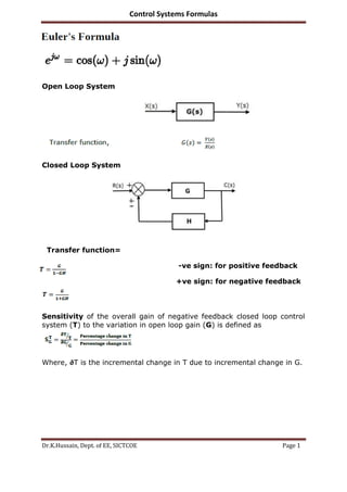
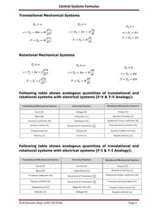
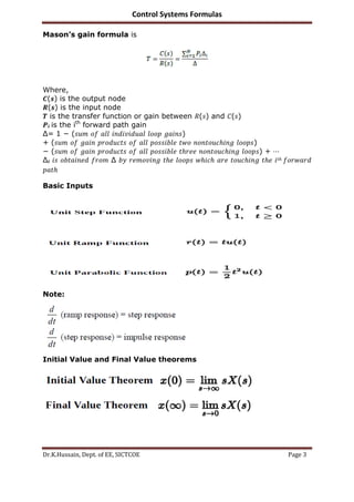
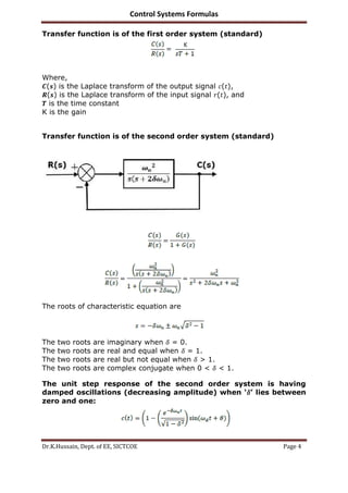
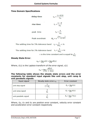
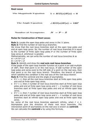
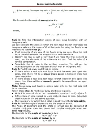
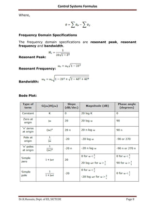
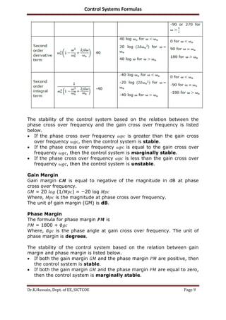
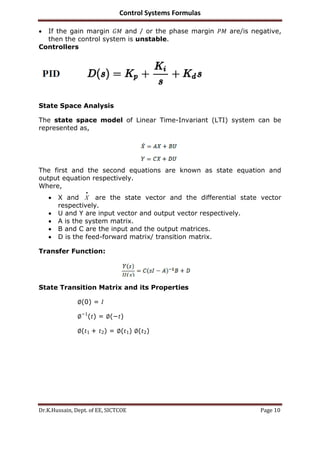
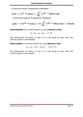
The document provides comprehensive formulas and principles related to control systems, including open and closed loop systems, transfer functions for both first and second order systems, and sensitivity analysis. It outlines rules for constructing root locus, frequency domain specifications like gain and phase margins, and introduces state space analysis along with controllability and observability tests. Additionally, it includes analogies between mechanical and electrical systems, error constants, and stability criteria.

1. Control Systems Formulas
Dr.K.Hussain, Dept. of EE, SICTCOE Page 1
Open Loop System
Closed Loop System
Transfer function=
-ve sign: for positive feedback
+ve sign: for negative feedback
Sensitivity of the overall gain of negative feedback closed loop control
system (T) to the variation in open loop gain (G) is defined as
Where, 𝞉T is the incremental change in T due to incremental change in G.

2. Control Systems Formulas
Dr.K.Hussain, Dept. of EE, SICTCOE Page 2
Translational Mechanical Systems
Rotational Mechanical Systems
Following table shows analogous quantities of translational and
rotational systems with electrical systems (F-V & T-V Analogy):
Following table shows analogous quantities of translational and
rotational systems with electrical systems (F-I & T-I Analogy):

3. Control Systems Formulas
Dr.K.Hussain, Dept. of EE, SICTCOE Page 3
Mason’s gain formula is
Where,
𝑪(𝒔) is the output node
𝑹(𝒔) is the input node
𝑻 is the transfer function or gain between 𝑅(𝑠) and 𝐶(𝑠)
𝑷𝒊 is the ith
forward path gain
Δ= 1 − (𝑠𝑢𝑚 𝑜𝑓 𝑎𝑙𝑙 𝑖𝑛𝑑𝑖𝑣𝑖𝑑𝑢𝑎𝑙 𝑙𝑜𝑜𝑝 𝑔𝑎𝑖𝑛𝑠)
+ (𝑠𝑢𝑚 𝑜𝑓 𝑔𝑎𝑖𝑛 𝑝𝑟𝑜𝑑𝑢𝑐𝑡𝑠 𝑜𝑓 𝑎𝑙𝑙 𝑝𝑜𝑠𝑠𝑖𝑏𝑙𝑒 𝑡𝑤𝑜 𝑛𝑜𝑛𝑡𝑜𝑢𝑐𝑕𝑖𝑛𝑔 𝑙𝑜𝑜𝑝𝑠)
− (𝑠𝑢𝑚 𝑜𝑓 𝑔𝑎𝑖𝑛 𝑝𝑟𝑜𝑑𝑢𝑐𝑡𝑠 𝑜𝑓 𝑎𝑙𝑙 𝑝𝑜𝑠𝑠𝑖𝑏𝑙𝑒 𝑡𝑕𝑟𝑒𝑒 𝑛𝑜𝑛𝑡𝑜𝑢𝑐𝑕𝑖𝑛𝑔 𝑙𝑜𝑜𝑝𝑠) + ⋯
Δ𝒊 𝑖𝑠 𝑜𝑏𝑡𝑎𝑖𝑛𝑒𝑑 𝑓𝑟𝑜𝑚 Δ 𝑏𝑦 𝑟𝑒𝑚𝑜𝑣𝑖𝑛𝑔 𝑡𝑕𝑒 𝑙𝑜𝑜𝑝𝑠 𝑤𝑕𝑖𝑐𝑕 𝑎𝑟𝑒 𝑡𝑜𝑢𝑐𝑕𝑖𝑛𝑔 𝑡𝑕𝑒 𝑖𝑡𝑕 𝑓𝑜𝑟𝑤𝑎𝑟𝑑
𝑝𝑎𝑡𝑕
Basic Inputs
Note:
Initial Value and Final Value theorems

4. Control Systems Formulas
Dr.K.Hussain, Dept. of EE, SICTCOE Page 4
Transfer function is of the first order system (standard)
Where,
𝑪(𝒔) is the Laplace transform of the output signal 𝑐(𝑡),
𝑹(𝒔) is the Laplace transform of the input signal 𝑟(𝑡), and
𝑻 is the time constant
K is the gain
Transfer function is of the second order system (standard)
The roots of characteristic equation are
The two roots are imaginary when 𝛿 = 0.
The two roots are real and equal when 𝛿 = 1.
The two roots are real but not equal when 𝛿 > 1.
The two roots are complex conjugate when 0 < 𝛿 < 1.
The unit step response of the second order system is having
damped oscillations (decreasing amplitude) when ‘𝛿’ lies between
zero and one:

5. Control Systems Formulas
Dr.K.Hussain, Dept. of EE, SICTCOE Page 5
Time Domain Specifications
Steady State Error:
Where, 𝐸(𝑠) is the Laplace transform of the error signal, 𝑒(𝑡)
The following table shows the steady state errors and the error
constants for standard input signals like unit step, unit ramp &
unit parabolic signals:
Where, 𝐾𝑝, 𝐾𝑣 and 𝐾𝑎 are position error constant, velocity error constant
and acceleration error constant respectively

6. Control Systems Formulas
Dr.K.Hussain, Dept. of EE, SICTCOE Page 6
Root Locus
Rules for Construction of Root Locus:
Rule 1: Locate the open loop poles and zeros in the ‘s’ plane.
Rule 2: Find the number of root locus branches.
We know that the root locus branches start at the open loop poles and
end at open loop zeros. So, the number of root locus branches 𝑵 is equal
to the number of finite open loop poles 𝑷 or the number of finite open
loop zeros 𝒁, whichever is greater.
Mathematically, we can write the number of root locus branches 𝑵 as
𝑵 = 𝑷 if 𝑷 ≥ 𝒁
𝑵 = 𝒁 if 𝑷 < 𝒁
Rule 3: Identify and draw the real axis root locus branches.
If the angle of the open loop transfer function at a point is an odd multiple
of 1800
, then that point is on the root locus. If odd number of the open
loop poles and zeros exist to the left side of a point on the real axis, then
that point is on the root locus branch. Therefore, the branch of points
which satisfies this condition is the real axis of the root locus branch.
Rule 4: Find the centroid and the angle of asymptotes.
 If 𝑃 = 𝑍, then all the root locus branches start at finite open loop poles
and end at finite open loop zeros.
 If 𝑃 > 𝑍, then 𝑍 number of root locus branches start at finite open loop
poles and end at finite open loop zeros and 𝑃 − 𝑍 number of root locus
branches start at finite open loop poles and end at infinite open loop
zeros.
 If 𝑃 < 𝑍, then 𝑃 number of root locus branches start at finite open loop
poles and end at finite open loop zeros and 𝑍 − 𝑃 number of root locus
branches start at infinite open loop poles and end at finite open loop
zeros.
So, some of the root locus branches approach infinity, when 𝑃 ≠ 𝑍.
Asymptotes give the direction of these root locus branches. The
intersection point of asymptotes on the real axis is known as centroid.
We can calculate the centroid 𝜶 by using this formula,

7. Control Systems Formulas
Dr.K.Hussain, Dept. of EE, SICTCOE Page 7
Rule 5: Find the intersection points of root locus branches with an
imaginary axis.
We can calculate the point at which the root locus branch intersects the
imaginary axis and the value of 𝑲 at that point by using the Routh array
method and special case (ii).
 If all elements of any row of the Routh array are zero, then the root
locus branch intersects the imaginary axis and vice-versa.
 Identify the row in such a way that if we make the first element as
zero, then the elements of the entire row are zero. Find the value of 𝑲
for this combination.
 Substitute this 𝑲 value in the auxiliary equation. You will get the
intersection point of the root locus branch with an imaginary axis.
Rule 6: Find Break-away and Break-in points.
 If there exists a real axis root locus branch between two open loop
poles, then there will be a break-away point in between these two
open loop poles.
 If there exists a real axis root locus branch between two open loop
zeros, then there will be a break-in point in between these two open
loop zeros.
Note: Break-away and break-in points exist only on the real axis root
locus branches.
Follow these steps to find break-away and break-in points.
 Write 𝐾 in terms of 𝑠 from the characteristic equation 1 + 𝐺(𝑠)𝐻(𝑠) = 0.
 Differentiate 𝐾 with respect to 𝑠 and make it equal to zero. Substitute
these values of 𝑠 in the above equation.
 The values of 𝑠 for which the 𝐾 value is positive are the break points.
Rule 7: Find the angle of departure and the angle of arrival.
The Angle of departure and the angle of arrival can be calculated at
complex conjugate open loop poles and complex conjugate open loop
zeros respectively.
The formula for the angle of departure ∅ 𝒅 is
∅ 𝑑 = 1800
− ∅
The formula for the angle of arrival ∅𝒂 is
∅ 𝑎 = 1800
+ ∅

8. Control Systems Formulas
Dr.K.Hussain, Dept. of EE, SICTCOE Page 8
Where,
Frequency Domain Specifications
The frequency domain specifications are resonant peak, resonant
frequency and bandwidth.
Resonant Peak:
Resonant Frequency:
Bandwidth:
Bode Plot:

9. Control Systems Formulas
Dr.K.Hussain, Dept. of EE, SICTCOE Page 9
The stability of the control system based on the relation between the
phase cross over frequency and the gain cross over frequency is listed
below.
 If the phase cross over frequency 𝜔𝑝𝑐 is greater than the gain cross
over frequency 𝜔𝑔𝑐, then the control system is stable.
 If the phase cross over frequency 𝜔𝑝𝑐 is equal to the gain cross over
frequency 𝜔𝑔𝑐, then the control system is marginally stable.
 If the phase cross over frequency 𝜔𝑝𝑐 is less than the gain cross over
frequency 𝜔𝑔𝑐, then the control system is unstable.
Gain Margin
Gain margin 𝑮𝑴 is equal to negative of the magnitude in dB at phase
cross over frequency.
𝐺𝑀 = 20 𝑙𝑜𝑔 (1/𝑀𝑝𝑐) = −20 log 𝑀𝑝𝑐
Where, 𝑀𝑝𝑐 is the magnitude at phase cross over frequency.
The unit of gain margin (GM) is dB.
Phase Margin
The formula for phase margin 𝑷𝑴 is
𝑃𝑀 = 1800 + ∅𝑔𝑐
Where, ∅𝑔𝑐 is the phase angle at gain cross over frequency. The unit of
phase margin is degrees.
The stability of the control system based on the relation between gain
margin and phase margin is listed below.
 If both the gain margin 𝐺𝑀 and the phase margin 𝑃𝑀 are positive, then
the control system is stable.
 If both the gain margin 𝐺𝑀 and the phase margin 𝑃𝑀 are equal to zero,
then the control system is marginally stable.

10. Control Systems Formulas
Dr.K.Hussain, Dept. of EE, SICTCOE Page 10
 If the gain margin 𝐺𝑀 and / or the phase margin 𝑃𝑀 are/is negative,
then the control system is unstable.
Controllers
State Space Analysis
The state space model of Linear Time-Invariant (LTI) system can be
represented as,
The first and the second equations are known as state equation and
output equation respectively.
Where,
 X and X

are the state vector and the differential state vector
respectively.
 U and Y are input vector and output vector respectively.
 A is the system matrix.
 B and C are the input and the output matrices.
 D is the feed-forward matrix/ transition matrix.
Transfer Function:
State Transition Matrix and its Properties
∅(0) = 𝐼
∅−1
(𝑡) = ∅(−𝑡)
∅(𝑡1 + 𝑡2) = ∅(𝑡1) ∅(𝑡2)

11. Control Systems Formulas
Dr.K.Hussain, Dept. of EE, SICTCOE Page 11
Controllability of a control system by using Kalman’s test:
The determinant of matrix 𝑄 𝑐 and if it is not equal to zero, then the
control system is controllable.
Observability of a control system by using Kalman’s test:
The determinant of matrix 𝑄 𝑜 and if it is not equal to zero, then the
control system is observable.