Downloaded 350 times


This document provides an overview of signal flow graphs and Mason's rule for calculating transfer functions from such graphs. It begins with definitions of key signal flow graph concepts like nodes, branches, paths, and loops. It then gives examples of constructing signal flow graphs from sets of simultaneous equations and converting block diagrams. Mason's rule is explained as providing the transfer function from a single formula involving the forward path gains and graph determinants, avoiding successive block diagram reductions. Finally, the document works through two examples applying Mason's rule to calculate transfer functions from given signal flow graphs.
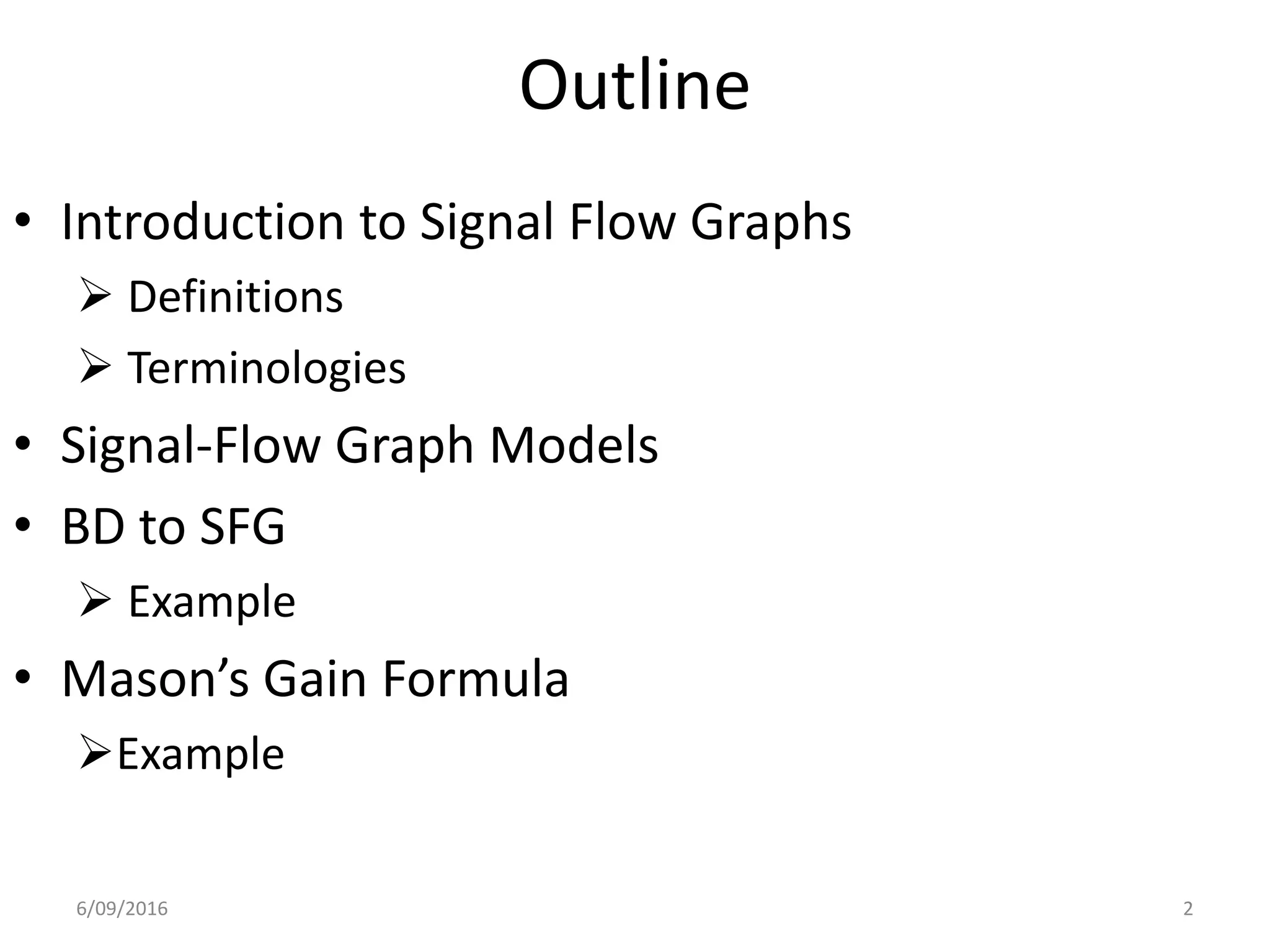
Overview of signal flow graphs and their components, including definitions, terminologies, and outline of the topics.
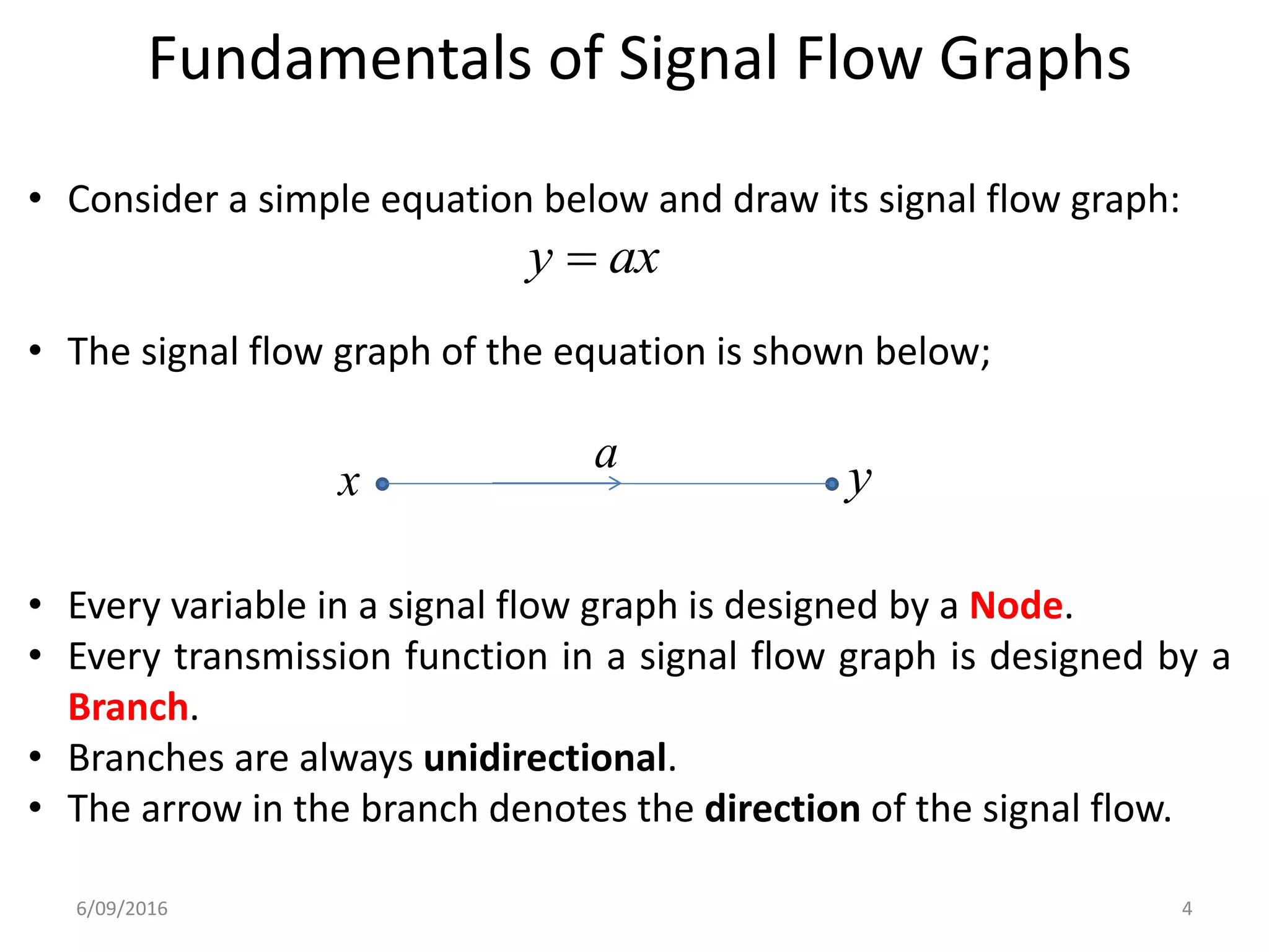
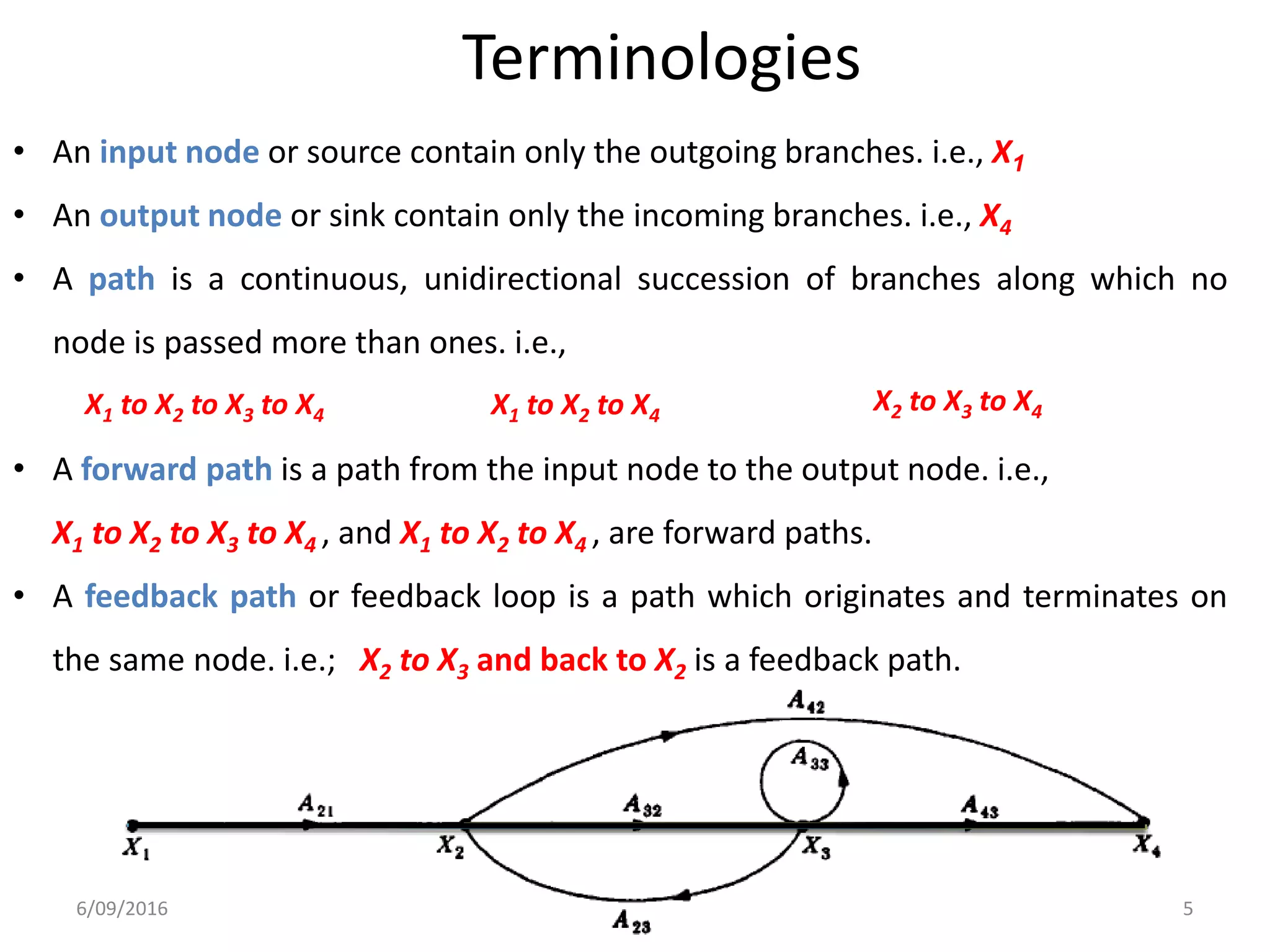
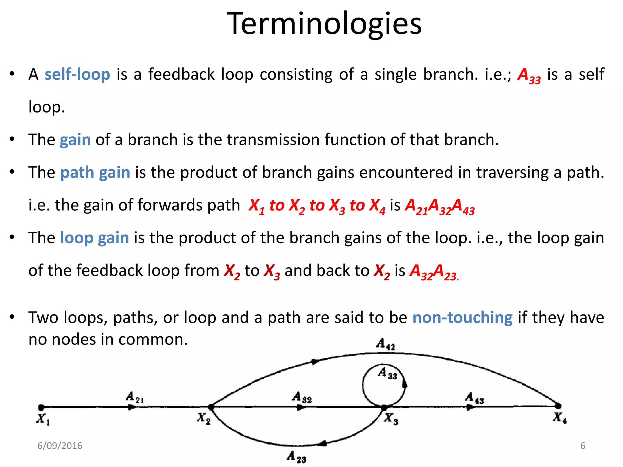
Definition and fundamental concepts of signal flow graphs, including nodes, branches, forward paths, feedback loops, and gains.
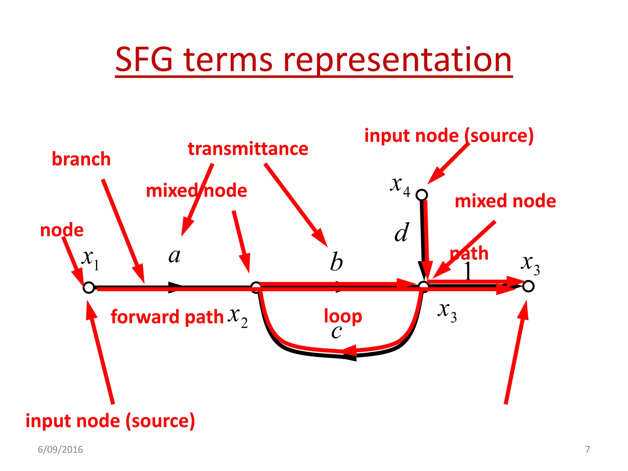
Visual representation of signal flow graph terms, including input nodes, forward paths, branches, and loops.
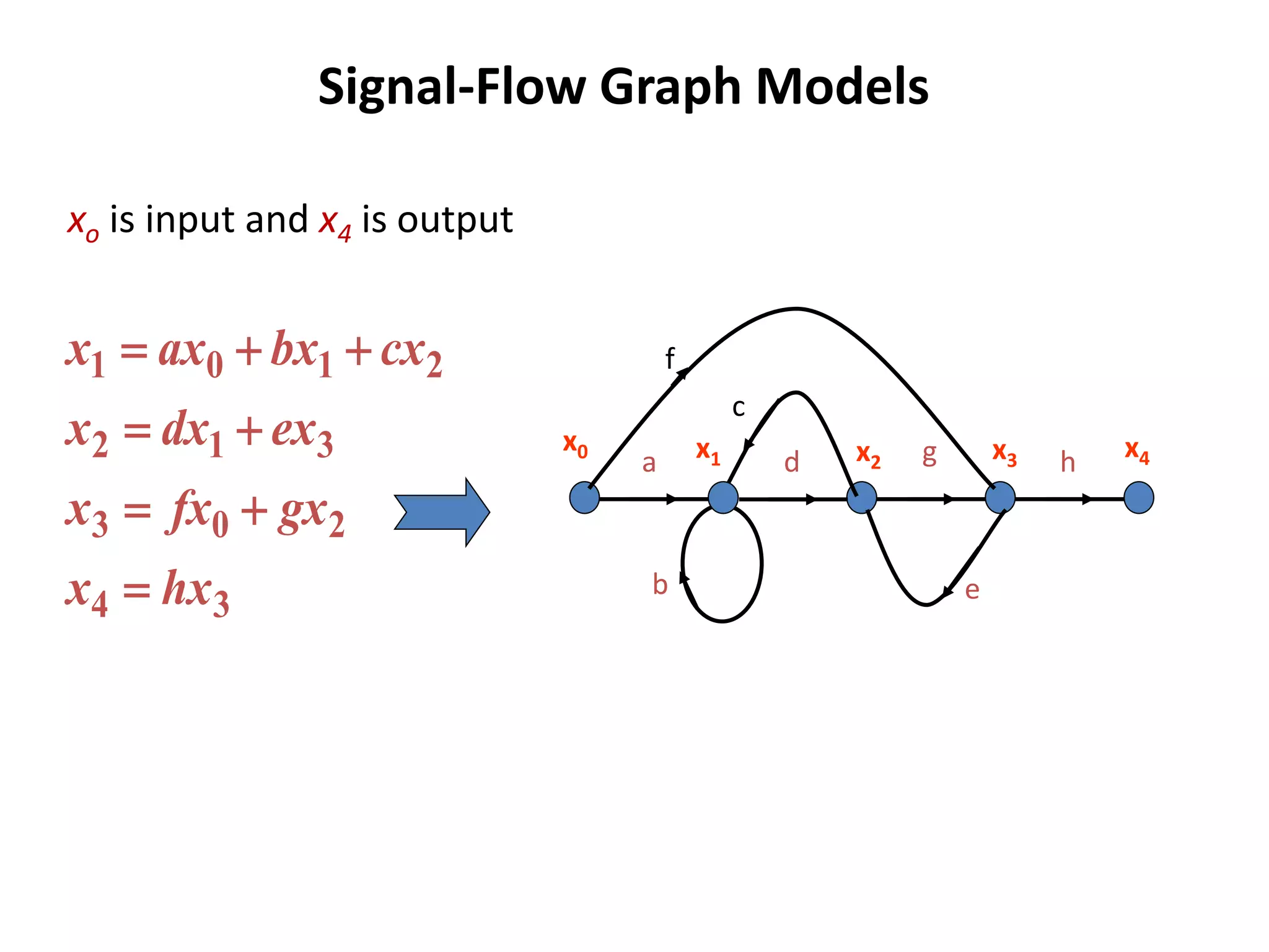
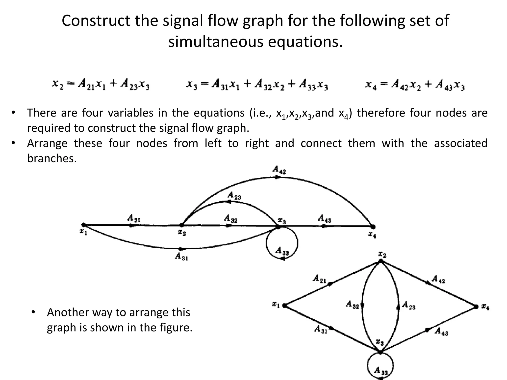
Demonstration of constructing signal flow graphs from simultaneous equations and their relations.
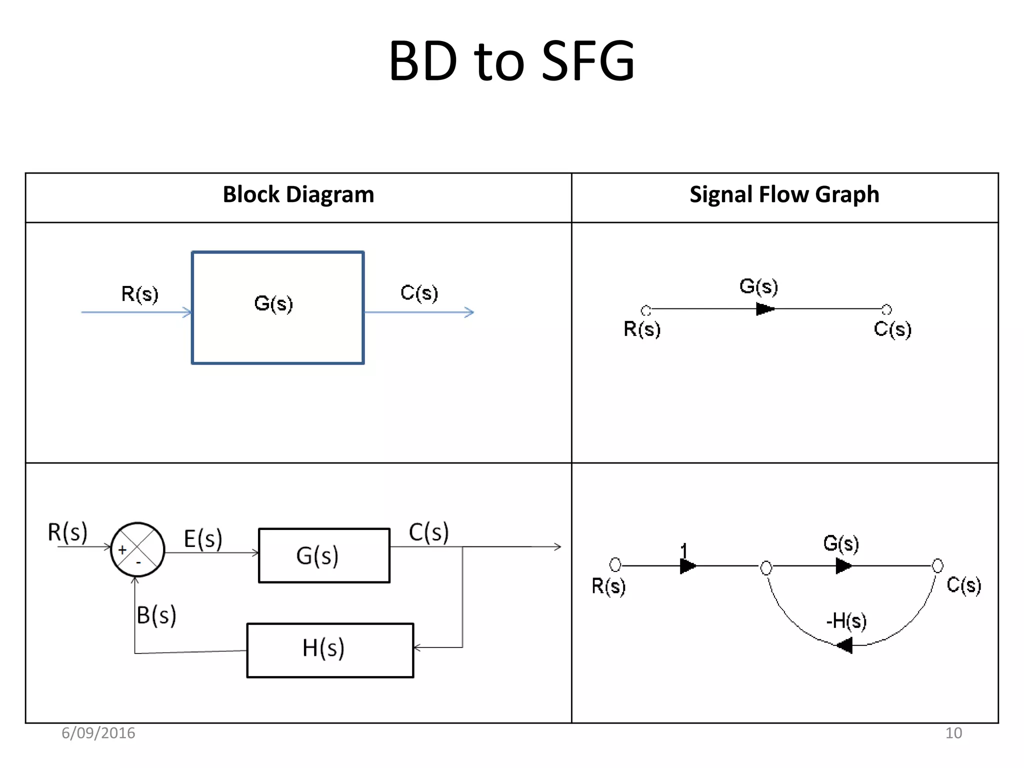
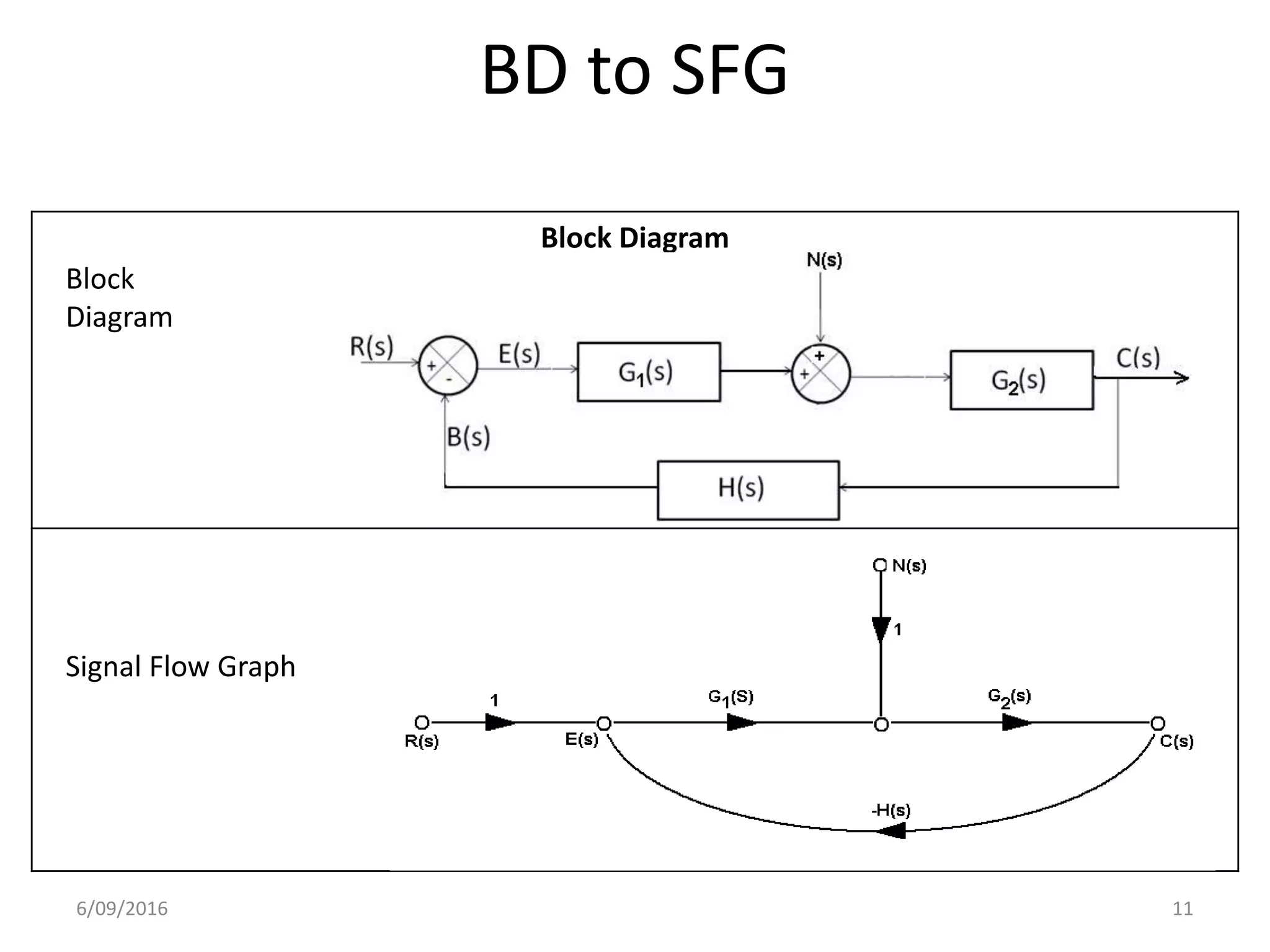
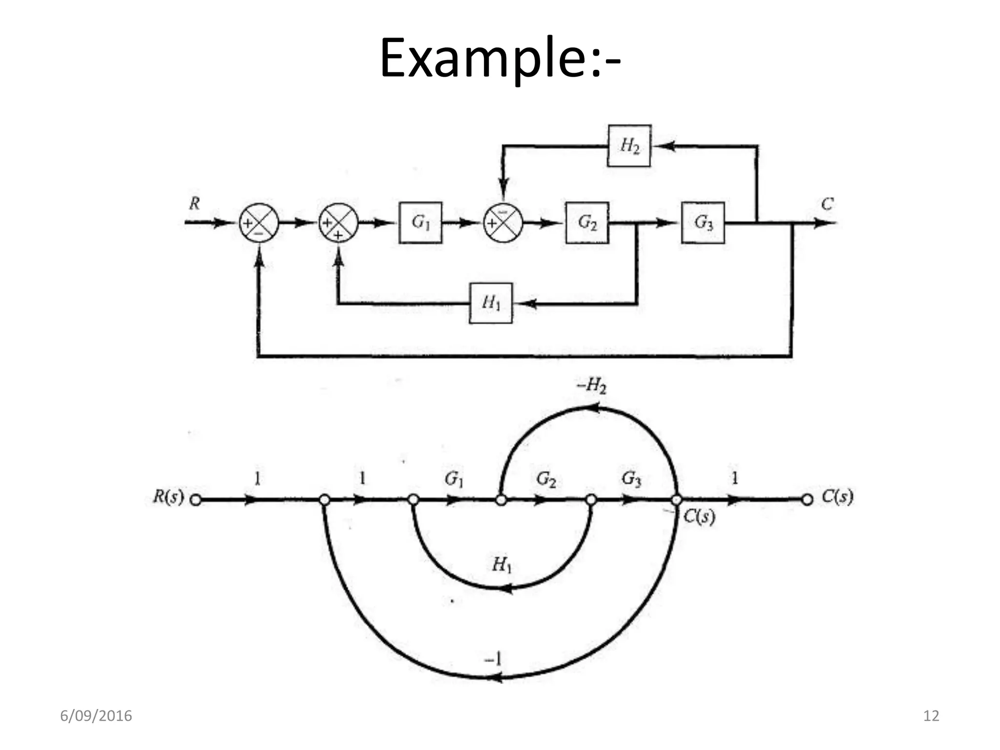
Concept of converting block diagrams to signal flow graphs with basic examples.
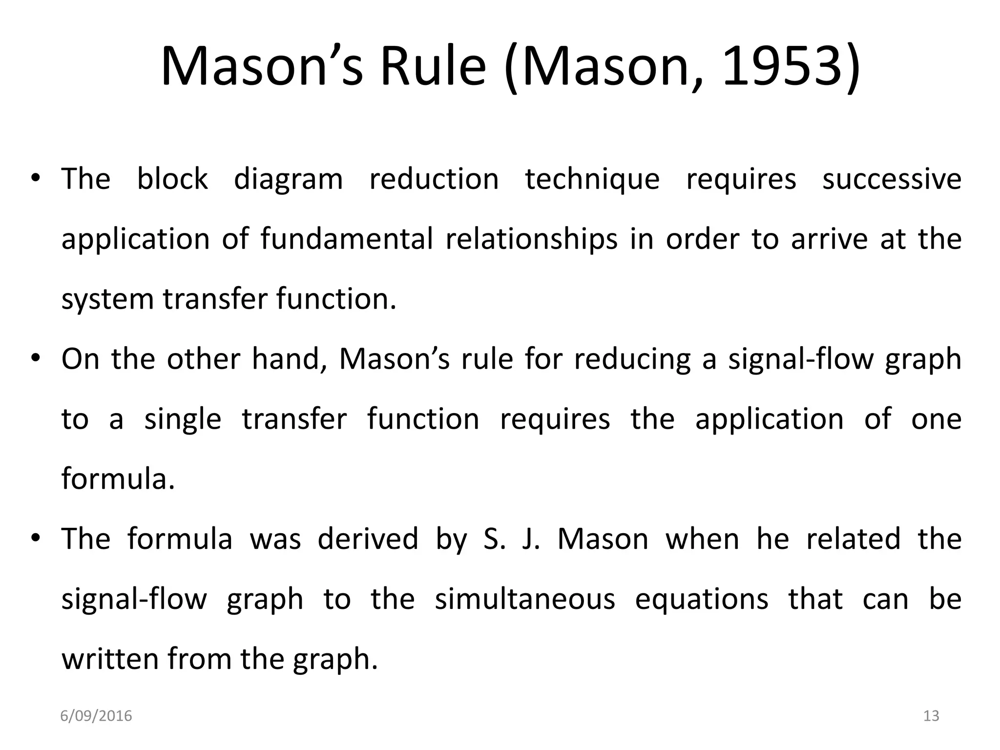
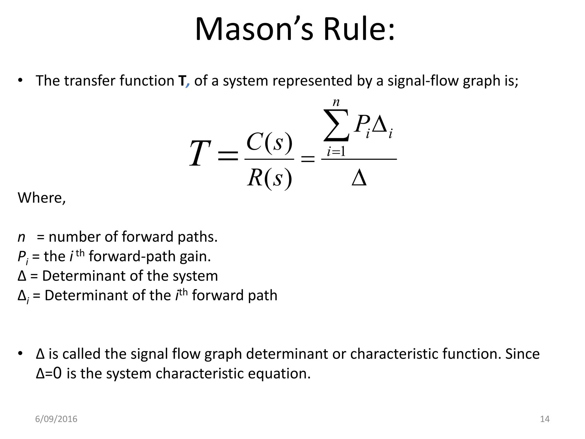
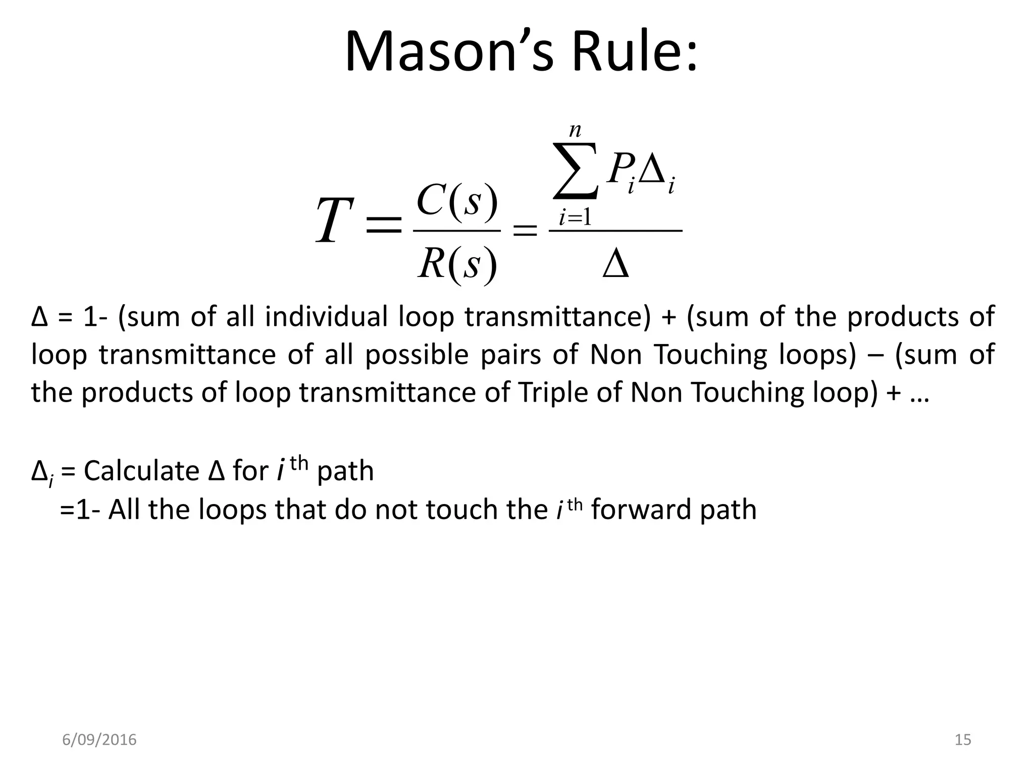
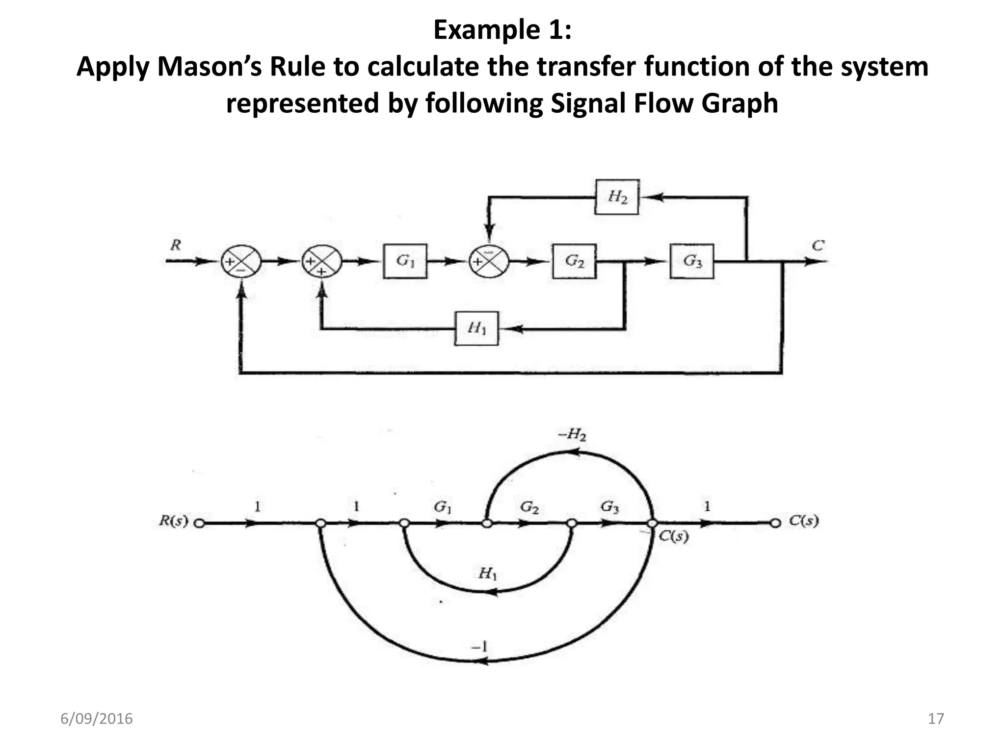
Introduction to Mason’s Rule for simplifying a signal flow graph and calculating transfer functions.
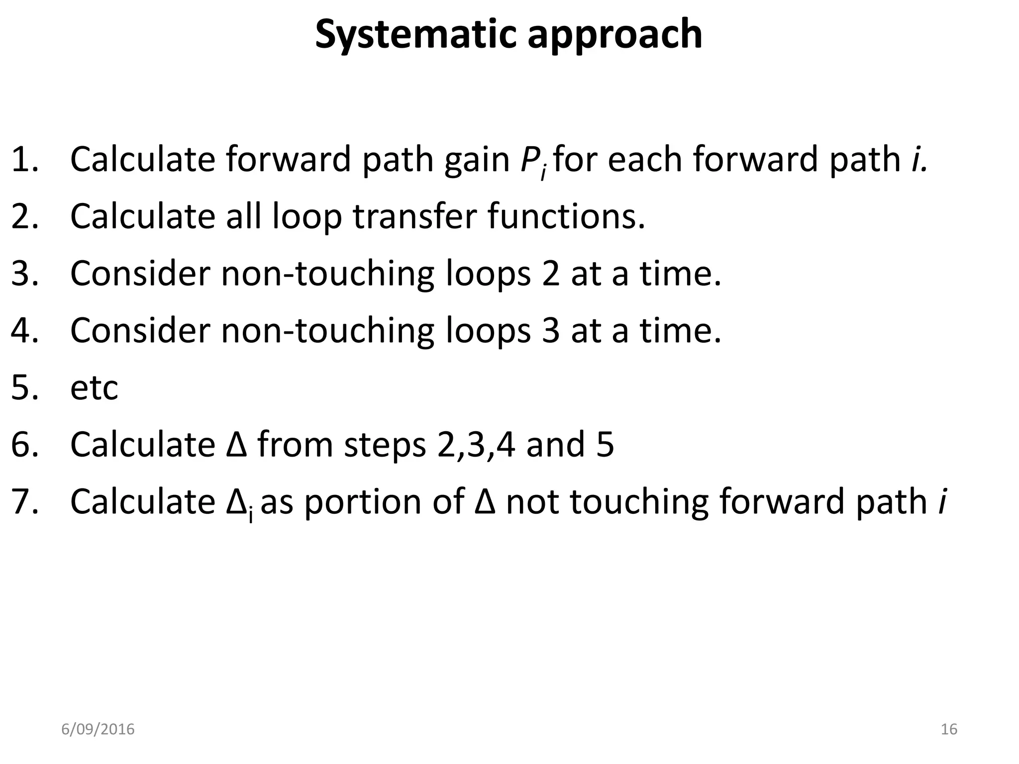
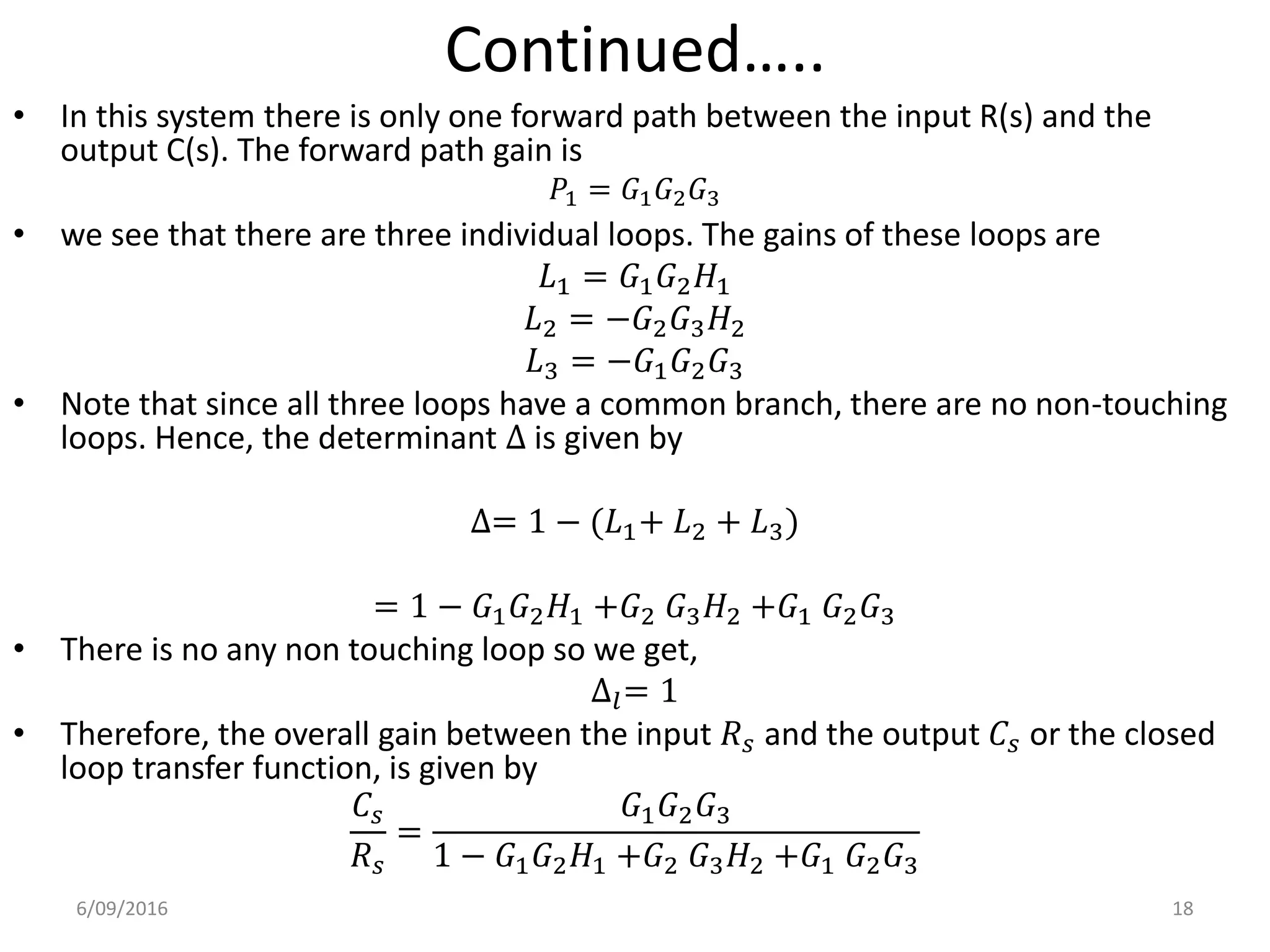
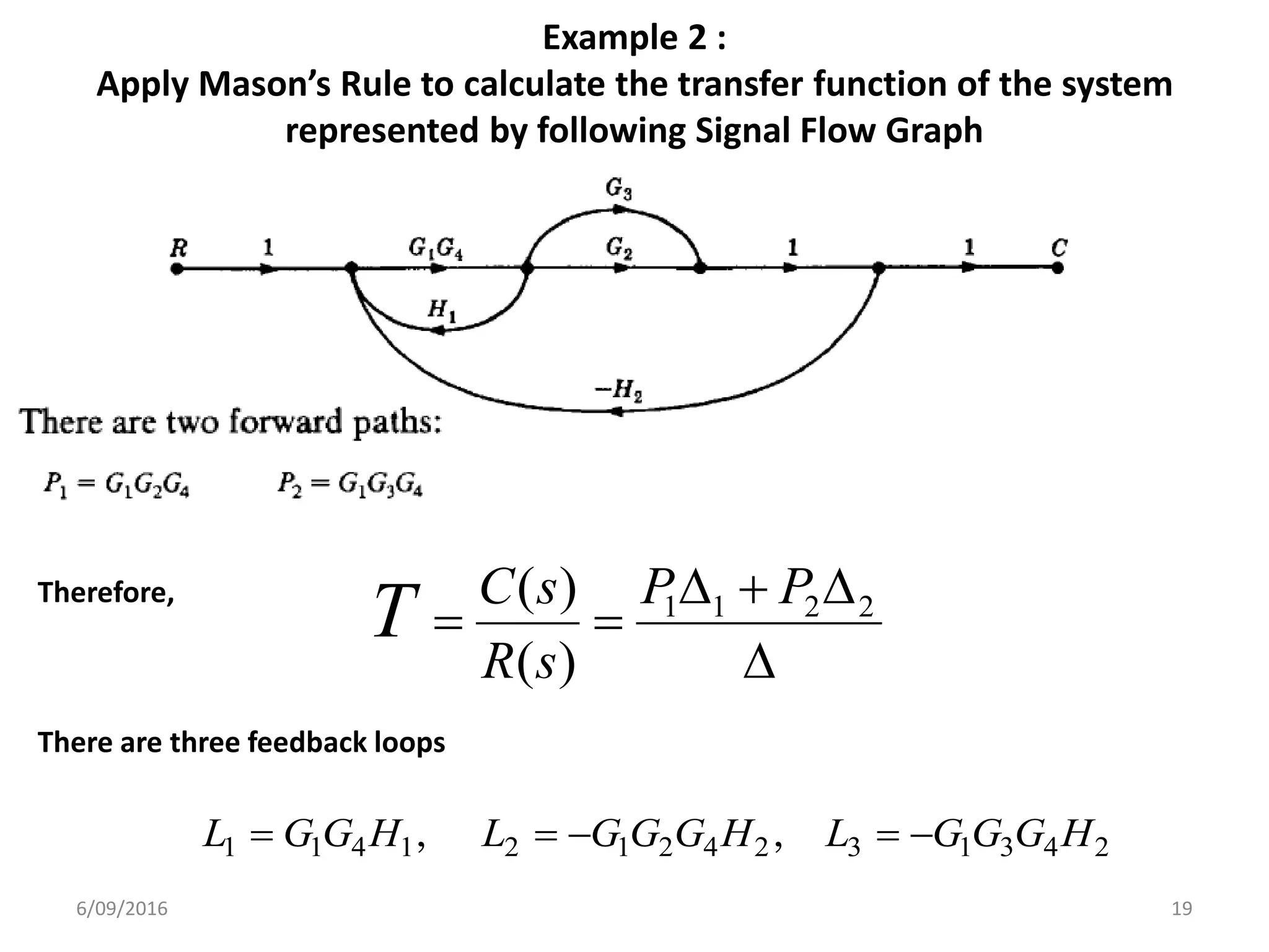
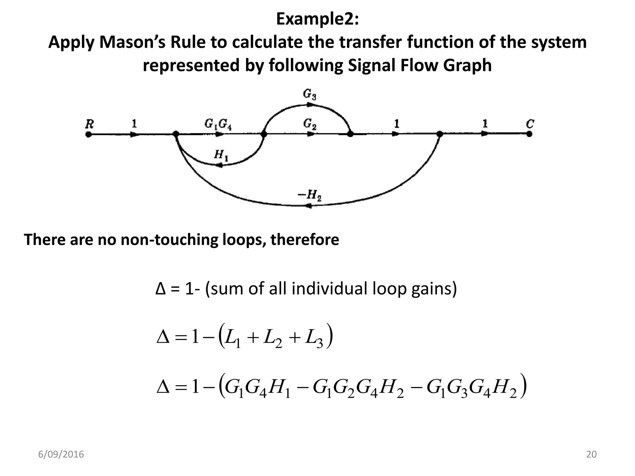
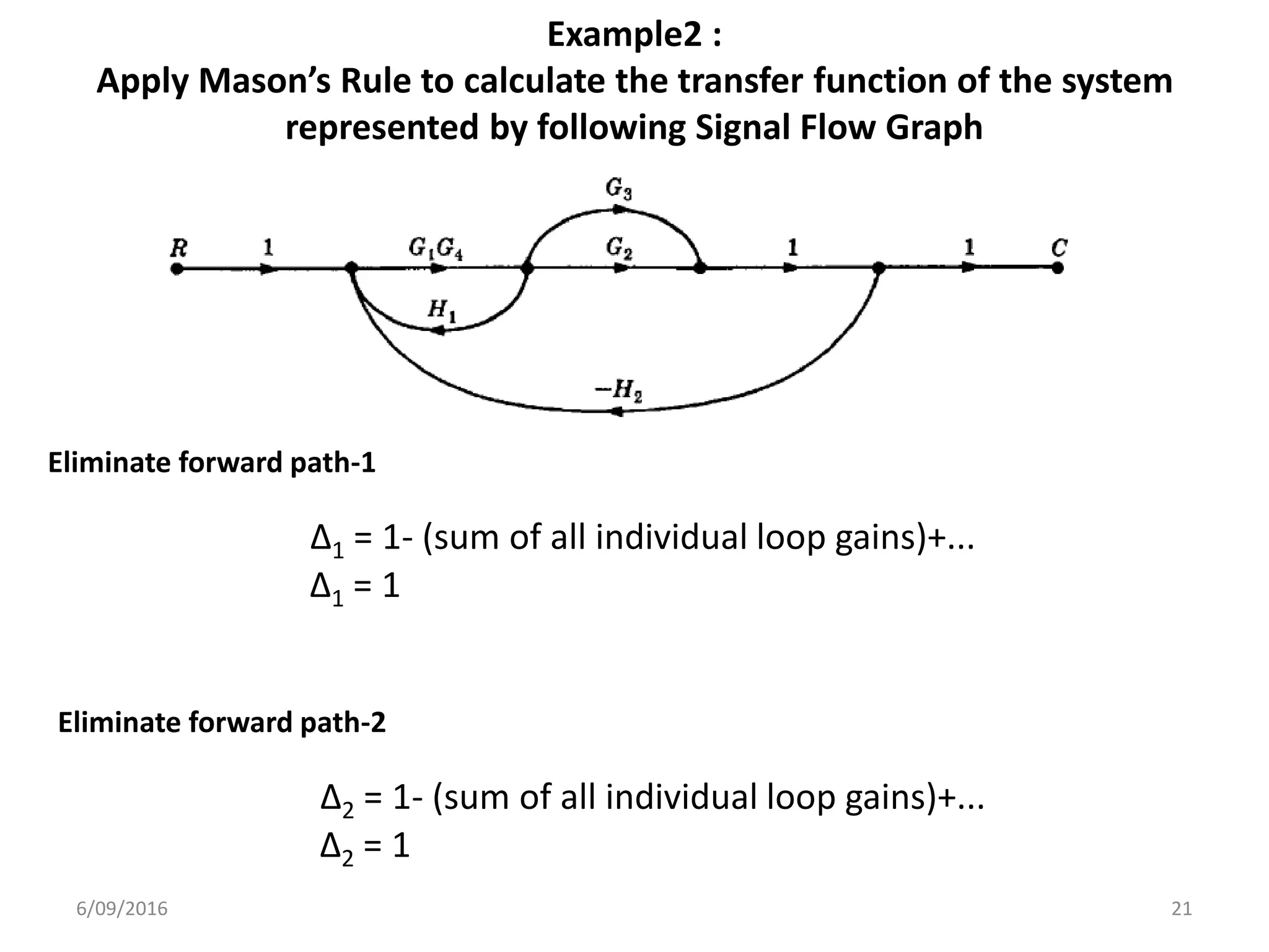
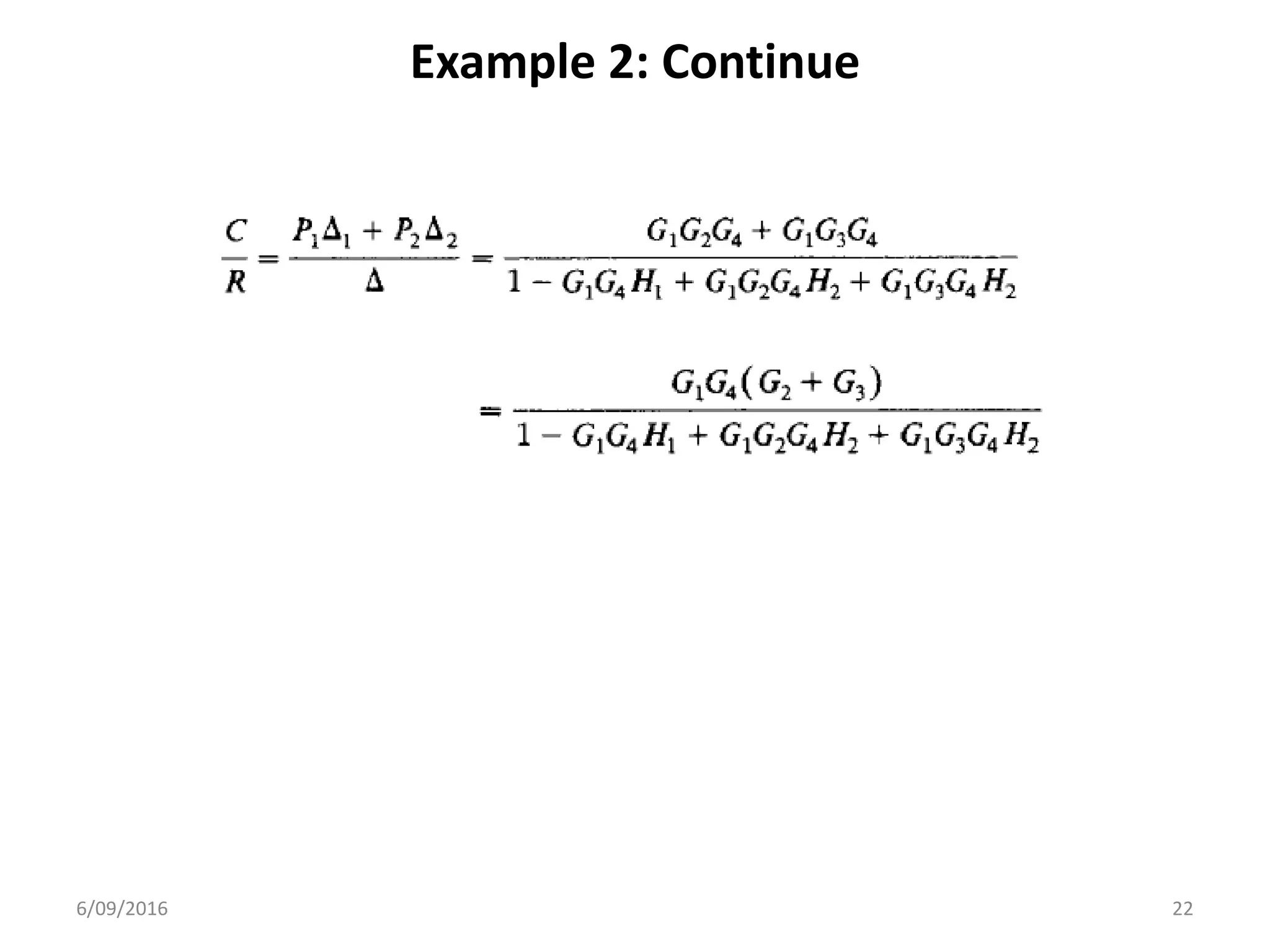
Step-by-step application of Mason's rule to calculate transfer functions using signal flow graphs with examples.
Closing remarks on the presentation.