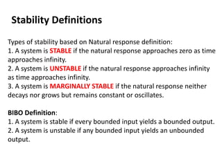
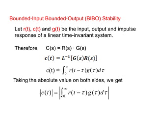
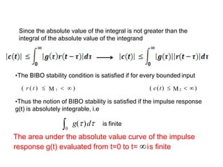
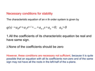
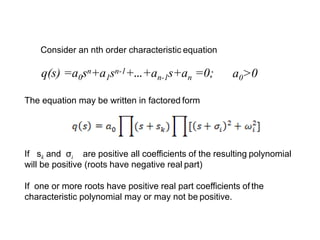
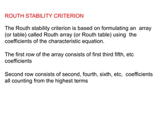
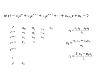
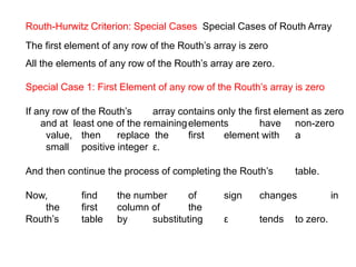
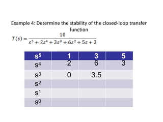
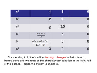
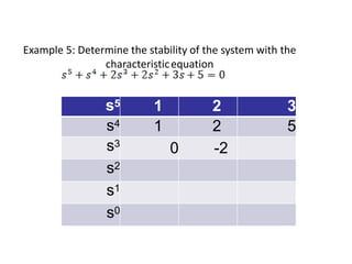
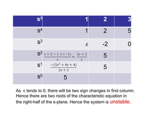
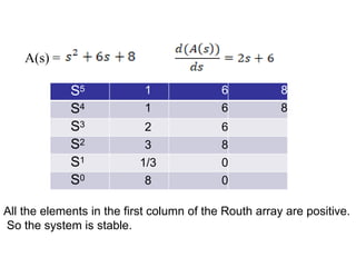
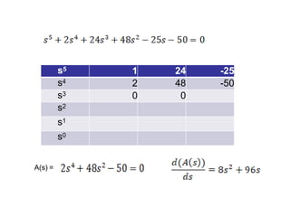
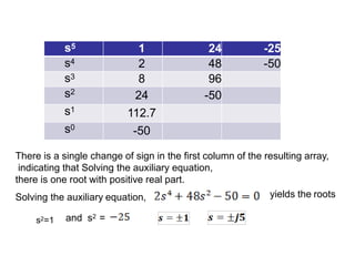
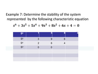
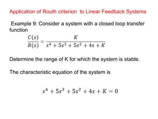
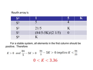
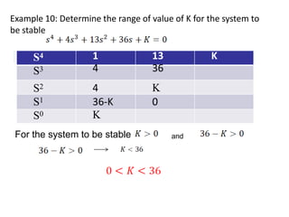
This presentation gives complete idea about definitions of stability, BIBO, Absolute and relative stability, Routh-Hurwitz Criterion, Special Cases and numerical examples.

1. Control System:
Stability and Routh Hurwitz Criterion
By
Dr.K.Hussain
Associate Professor & Head
Dept. of EE, SITCOE

2. Stability Definitions
Types of stability based on Natural response definition:
1. A system is STABLE if the natural response approaches zero as time
approaches infinity.
2. A system is UNSTABLE if the natural response approaches infinity
as time approaches infinity.
3. A system is MARGINALLY STABLE if the natural response neither
decays nor grows but remains constant or oscillates.
BIBO Definition:
1. A system is stable if every bounded input yields a bounded output.
2. A system is unstable if any bounded input yields an unbounded
output.

3. Bounded-Input Bounded-Output (BIBO) Stability
Let r(t), c(t) and g(t) be the input, output and impulse
response of a linear time-invariant system.
Therefore C(s) = R(s) ∙ G(s)

r(t  )g( )dc(t) = 0
Taking the absolute value on both sides, we get

c(t)  0
r(t   )g( )d

4. Since the absolute value of the integral is not greater than the
integral of the absolute value of the integrand
•The BIBO stability condition is satisfied if for every bounded input
( r ( t )  M 1   ) ( c(t)  M 2  )
•Thus the notion of BIBO stability is satisfied if the impulse response
g(t) is absolutely integrable, i.e
g()d0
is finite
. The area under the absolute value curve of the impulse
response g(t) evaluated from t=0 to t= is finite

7. ABSOLUTE STABILITY AND RELATIVE STABILITY
ABSOLUTE STABILITY
Absolute stability is a qualitative measure of stability. It
refers to the condition of whether the system is stable
or unstable
RELATIVE STABILITY
Once the system is found to be stable, it is of interest to
determine how stable it is, and this degree of stability is
a measure of relative stability. Relative stability is a
quantitative measure of how fast transients die out in
the system.

8. RELATIVE STABILITY
Relative stability measurement- relative settling time of
each unit or pair of units
Relative settling time of complex conjugate pole is
inversely proportional to the real part of the roots
Root or pair of roots move farther away from imaginary
axis, the relative stability of the system improves

9. Necessary conditions for stability
The characteristic equation of an n th order system is given by
q(s) =a0sn+a1sn-1+…+an-1s+an =0; a0>0
1.All the coefficients of its characteristic equation be real and
have same sign.
2.None of the coefficients should be zero
However, these conditions are necessary not sufficient, because it is quite
possible that an equation with all its coefficients non-zero and of the same
sign may not have all the roots in the left-half of the s-plane.

10. The equation may be written in factored form
If sk and σi are positive all coefficients of the resulting polynomial
will be positive (roots have negative real part)
If one or more roots have positive real part coefficients of the
characteristic polynomial may or may not be positive.
Consider an nth order characteristic equation
q(s) =a0sn+a1sn-1+…+an-1s+an =0; a0>0

11. ROUTH STABILITY CRITERION
The Routh stability criterion is based on formulating an array
(or table) called Routh array (or Routh table) using the
coefficients of the characteristic equation.
The first row of the array consists of first third fifth, etc
coefficients
Second row consists of second, fourth, sixth, etc, coefficients
all counting from the highest terms

12. .

13. Example 1: Investigate whether the following systems represented by the
characteristic equations are stable or not.
s5
 s4
 6s3
12s2
18s  6  0
s5
S4
s3
s2
1 6 18
1 12 6
-6 12 0
14 6
s1
14.5
7
0
s0 6
There are two sign changes in
the first column of the Routh
array.
Hence there are two roots of
the characteristic equation in
the right-half of the s-plane.
Hence the system is unstable

14. s4
 2s3
10s2
 8s  3  0
s4 1 10 3
s3 2 8
s2
s1
s0
2
210 18
 6
2
2  3 1 0
 3
6  8  2  3
6
 7 6
6  0  2  0
 0
73 60
 3
7
All the elements in the first column of the Routh array are positive.
So the system is stable
Example 2: Investigate whether the following systems represented by the
characteristic equations are stable or not.

15. s6
 2s5
 8 s4
 1 5 s 3
s6 1 8
s5 2 15 16
s4 0.5 12 16
s3 -33 -48
s2 11.27 16
s1 -1.16 0
s0 16
There are four sign changes in the elements of first column of the Routh
array.
Hence there are four roots of the characteristic equation in the right-half of the
s-plane.
Hence the system is unstable
 20s2
 1 6 s  1 6  0
20 16
Example 3: Investigate whether the following systems represented by the
characteristic equations are stable or not.

16. Routh-Hurwitz Criterion: Special Cases Special Cases of Routh Array
The first element of any row of the Routh’s array is zero
All the elements of any row of the Routh’s array are zero.
Special Case 1: First Element of any row of the Routh’s array is zero
If any row of the Routh’s array contains only the first element as zero
and at least one of the remainingelements have non-zero
value, then replace the first element with a
small positive integer ε.
And then continue the process of completing the Routh’s table.
Now, find the number of sign changes in
the first column of the
Routh’s table by substituting ε tends to zero.

17. Example 4: Determine the stability of the closed-loop transfer
function
s5 1 3 5
s4 2 6 3
s3 0 3.5
s2
s1
s0

18. s5 1 3 5
s4 2 6 3
s3
𝜀 3.5 0
s2 3 0
s1 0 0
s0 3 0 0
For 𝜀 tending to 0, there will be two sign changes in first column.
Hence there are two roots of the characteristic equation in the right-half
of the s-plane. Hence the system is unstable.

19. 1 2 3
1 2 5
0
Example 5: Determine the stability of the system with the
characteristicequation
s5 1 2 3
s4 1 2 5
s3
0 -2
s2
s1
s0

20. s5 1 2 3
s4 1 2 5
s3
𝜀 -2 0
s2
5
s1
5
s0
5
As ϵ tends to 0, there will be two sign changes in first column.
Hence there are two roots of the characteristic equation in
the right-half of the s-plane. Hence the system is unstable.

21. ALTERNATE METHOD:
Transform the characteristic equation by replacing s by
and apply Routh’s test. Let the equation be
Replacing s by 1/z we have

22. z5 5 2 1
z4 3 2 1
z3
-1.33 -0.66 0
z2
0.5 1
z1
2
z0
1
There are two sign changes in first column. Hence
there are two roots of the characteristic equation in the
right-half of the s-plane. Hence the system is unstable

23. Special Case 2: All the Elements of any row of the
Routh’s array arezero.
This condition indicates that there are symmetrically located roots in the
s-plane, which may be
Pair of real roots with opposite sign
Pair of conjugate roots on the imaginary axis
Complex conjugate roots forming quadrates
Polynomial whose coefficients are the elements above the row of zeros
are called auxiliary equation.
Order of the auxiliary equation is always even.
To proceed with Routh’s table, replace the row of zeros with coefficient of
polynomial obtained by taking first derivative of the auxiliary polynomial.

24. Example 6: Determine the number of right hand plane poles in the closed-loop transfer
function
S5 1 6 8
s4 7 42 56
s4 1 6 8
s3 0 0
s2
s1
s0

25. A(s) =
S5 1 6 8
S4 1 6 8
S3 2 6
S2 3 8
S1 1/3 0
S0 8 0
All the elements in the first column of the Routh array are positive.
So the system is stable.

26. s5 1 24 -25
s4 2 48 -50
s3 0 0
s2
s1
s0
A(s) =

27. s5 1 24 -25
s4 2 48 -50
s3 8 96
s2
24 -50
s1
112.7
s0
-50
There is a single change of sign in the first column of the resulting array,
indicating that Solving the auxiliary equation,
there is one root with positive real part.
Solving the auxiliary equation, yields the roots
s2=1 and s2 =

28. Example 7: Determine the stability of the system
represented by the following characteristic equation
S6 1 5 8 4
S5 3 9 6
S4 2 6 4
S3 0 0

29. S6 1 5 8 4
S5 3 9 6
S4 2 6 4
S3 2 3
S2 3 4
S1 1/3 0
S0 4

30. Factorizing A(s) we h ve
Solving the auxiliary we have
a
There are two pairs of non repeated roots on the
imaginary axis, hence the system is marginally stable

31. Example 8: Using the Routh criterion check whether the system
representedby the following characteristic equation is stable or
not. Determinethe frequency of oscillations if any.
S4 1 6 8
S3 2 8
S2 2 8
S1 0 0
S0

32. S4 1 6 8
S3 2 8
S2 2 8
S1 4 0
S0 8
Solving the auxiliary we have
So the system oscillates with frequency ω= 2 rad/sec

33. Application of Routh criterion to Linear Feedback Systems
Example 9: Consider a system with a closed loop transfer
function
Determine the range of K for which the system is stable.
The characteristic equation of the system is

34. S4 1 5 K
S3 5 4
S2 21/5 K
S1 (84/5-5K)/(2 1/5) 0
S0 K
Routh array is
For a stable system, all elements in the first column should be
positive. Therefore

35. Example 10: Determine the range of value of K for the system to
be stable
S4 1 13 K
S3 4 36
S2 4 K
S1 36-K 0
S0 K
For the system to be stable and

36. THANK YOU