Downloaded 736 times
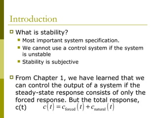
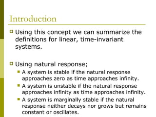
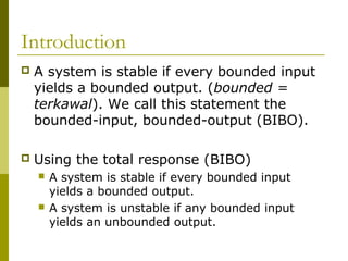
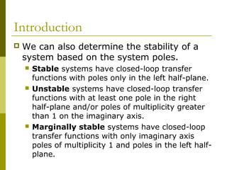

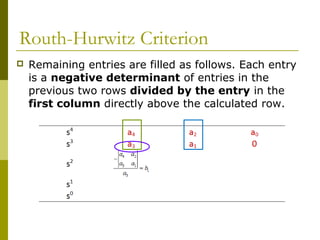
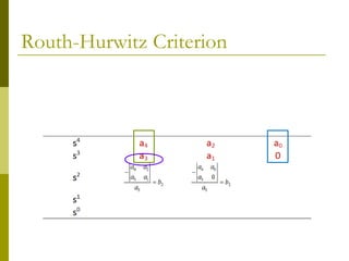
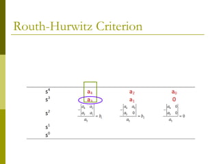
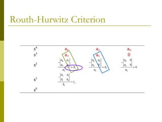
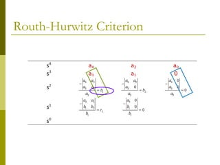
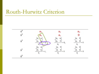
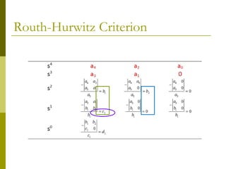
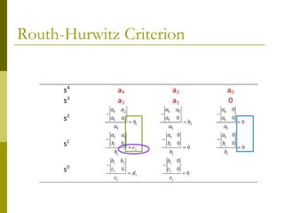
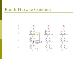
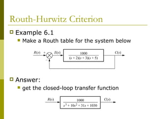
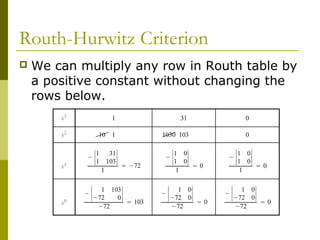
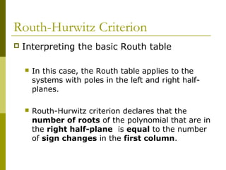
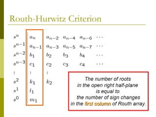
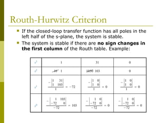
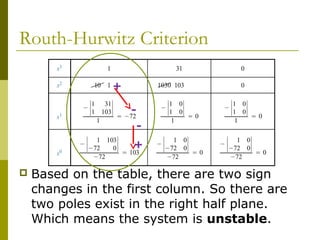
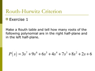
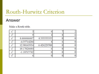
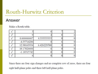
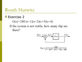
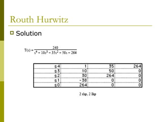
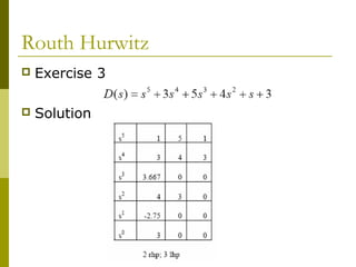
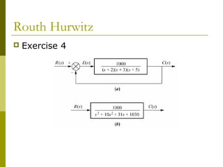
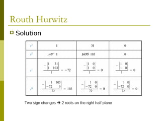
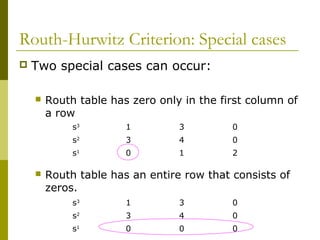
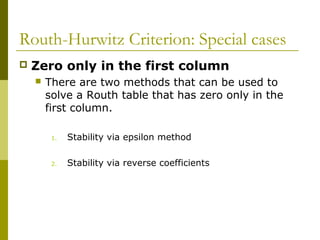
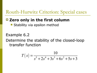
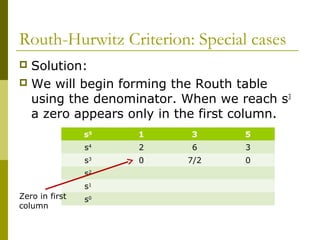
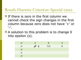
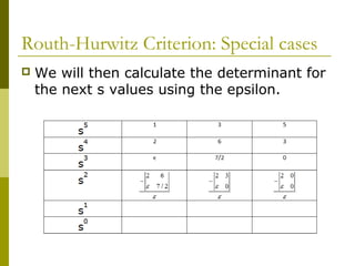
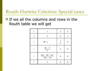
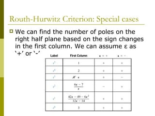
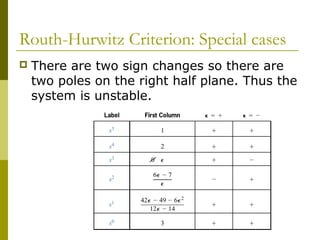
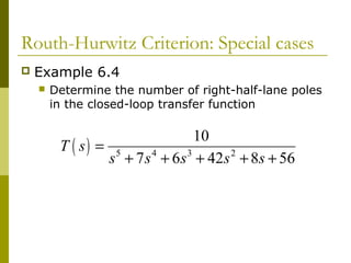
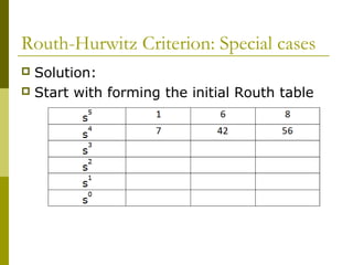
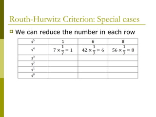
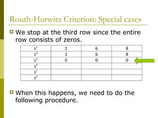
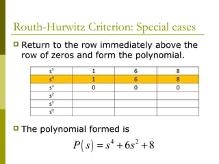
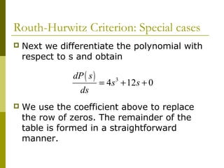
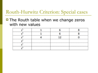
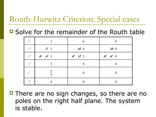
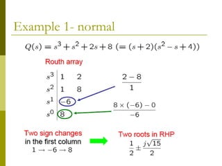
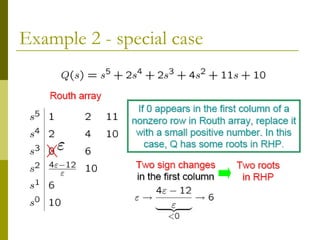
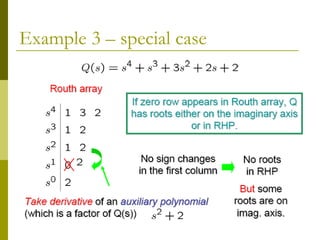
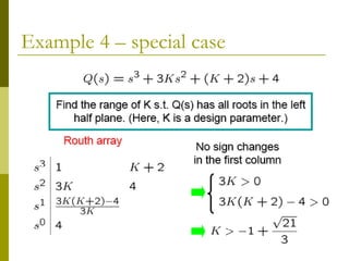

This document discusses stability analysis of control systems using transfer functions and the Routh-Hurwitz criterion. It begins by defining stability and describing different types of system responses. The key points are: 1) The Routh-Hurwitz criterion can determine stability by analyzing the signs in the first column of a constructed Routh table, with changes in sign indicating right half-plane poles and instability. 2) Special cases like a zero only in the first column or an entire row of zeros require alternative methods like the epsilon method or reversing coefficients. 3) Examples demonstrate applying the Routh-Hurwitz criterion to determine stability for different polynomials, including handling special cases. Exercises also have readers practice stability analysis using
![Reduction of multiple subsystem [compatibility mode]](https://cdn.slidesharecdn.com/ss_thumbnails/reductionofmultiplesubsystemcompatibilitymode-110418075355-phpapp01-thumbnail.jpg?width=640&height=640&fit=bounds)


![Roth_herwitz_stability_criterion-[1].pdf](https://cdn.slidesharecdn.com/ss_thumbnails/rothherwitzstabilitycriterion1-251026051926-6a7e967e-thumbnail.jpg?width=640&height=640&fit=bounds)


