The document summarizes a lecture on regression analysis and curve fitting in mathematical modelling. It introduces regression analysis and its applications. It describes different regression techniques like linear, nonlinear, polynomial and multiple regression. It provides examples of fitting linear and polynomial curves to data using MATLAB. It discusses assessing the goodness of fit using metrics like residual norm and coefficient of determination.

1. Data Approximation in Mathematical
Modelling: Regression Analysis and
Curve Fitting
DR. SUMMIYA PARVEEN
Department of Mathematics
COLLEGE OF ENGINEERING ROORKE (COER)
ROORKEE
summiyaparveen82@gmail.com
Dr. Summiya Parveen 1

2. Outline of the lecture:
Introduction of Regression
Application of Regression
Regression Techniques
Types of Regression
Goodness of fit
MATLAB/MATHEMATICA
implementation with some example
Dr. Summiya Parveen 2

3. Regression
Regression analysis is a form of predictive modelling technique which investigates the
relationship between a dependent (target) and independent variable (s) (predictor). This
technique is used for forecasting, time series modelling and finding the casual effect
relationship between the variables.
Regression analysis is an important tool for modelling and analysing data. Here, we fit a
curve / line to the data points in such a manner that the differences between the distances of
data points from the curve or line is minimized.
Independent variable (x)
Dependentvariable(y)
Year Research &
development
Investment
(millions)
Annual Profit
(millions)
2011 2 20
2012 3 25
2013 5 34
2014 4 30
2015 11 40
2016 5 31
2017 6 25
2019 15 ?
2020 ? 50
Dr. Summiya Parveen 3

4. Applications of Regression Analysis
Agricultural Science
Industrial Production
Environment Science
Business
Health Care
Dr. Summiya Parveen 4

5. Regression Techniques
There are various types of regression techniques available
to make predictions. These techniques are mostly driven
by three metrics (number of independent variables, type of
dependent variables and shape of regression line).
Dr. Summiya Parveen 5

6. Commonly used Types of Regression
Linear Regression
Non - Linear Regression
Polynomial Regression
Multiple Regression
Dr. Summiya Parveen 6

7. Linear Regression
The output of a simple
regression is the coefficient a1
and the constant a0. The
equation is then:
y = a0 + a1 x + e
where
e is the residual error.
a1 is the per unit change in the
dependent variable for each unit
change in the independent
variable. Mathematically:
Dr. Summiya Parveen 7

8. Non-linear Regression
Non-linear functions can also be fitted as regressions.
For examples Power function , Logarithmic function and
Exponential functions.
Dr. Summiya Parveen 8

9. Polynomial Regression
Polynomial equation in m degree
may be taken as :
y = a0 + a1x + a2x2 +....amxm+ e
Here a0 , a1, ……. am
are constant and
e = residual error
Dr. Summiya Parveen 9

10. Multiple Linear Regression
A useful extension of linear regression is the case where
dependent variable y is a linear function of two or more
independent variables
e.g
y = ao + a1x1 + a2x2
We follow the same procedure
y = ao + a1x1 + a2x2 + e
where
e= residual error .
Dr. Summiya Parveen 10

11. Linear Regression
Independent variable (x)
Dependentvariable(y)
The output of a regression is a function that predicts the
dependent variable based upon values of the independent
variable.
Linear regression fits a straight line to the data.
y = a0 + a1 x + e
a0 (y intercept)
a1 = slope
= ∆y/ ∆x
e
Dr. Summiya Parveen 11

12. 12
Fitting a straight line to a
set of paired observations:
(x1, y1), (x2, y2),…,(xn, yn)
yi = a0 + a1 xi + ei
ei = yi - a0 - a1 xi
Here
yi : measured value
ei : error
a1 : slope
a0 : intercept
Linear Regression
e Error
Line equation
y = a0 + a1 x
Dr. Summiya Parveen

13. Best strategy is to minimize the sum of the squares of the residual errors
between the measured-y and the y calculated with the linear model:
Here we need to compute a0 and a1 such that Sr is minimized.









n
i
iir
n
i
modelimeasuredi
n
i
ir
xaayS
yy
eS
1
2
10
1
2
,,
1
2
)(
)(
e Error
Dr. Summiya Parveen 13

14. Least-Square Fit of a Straight Line
  00)(2
00)(2
2
101
1
101






 
 
iiiiiioi
r
iiioi
o
r
xaxaxyxxaay
a
S
xaayxaay
a
S
Normal equations which can
be solved simultaneously
 
    iiii
ii
xyaxax
yaxna
naa






1
2
0
10
00
(2)
(1)
Since
 

n
i
ii
n
i
ir xaayeS
1
2
10
1
2
)(:errorMinimize
Dr. Summiya Parveen 14

15.  
xayaa
xxn
yxyxn
a
ii
iiii
100
221
asexpressedbecan 



 
  
Solving equations (1) and (2) we get
Mean values
Dr. Summiya Parveen 15

16. To understand how well the X predicts the Y, we evaluate
Variability in the Y
variable
SSR –> Regression
Variability that is
explained by the
relationship b/w X & Y
+
SSE –> Unexplained
Variability, due to
factors then the
regression
-------------------------------
SST –> Total variability
about the mean
Correlation
Coefficient
r – Strength of the
Relationship
between Y and X
variables
Standard
Error
St Deviation of
error around
the Regression
Line
Residual
Analysis
Validation of
Model
Coefficient of Determination
R Sq - Proportion of explained
variation
Test for Linearity
Significance of the
Regression Model
i.e. Linear Regression
Model
“Goodness” of fit
Dr. Summiya Parveen 16

17. Independent variable (x)
Dependentvariable(y) Population mean: y
y
X
SSE
SSR
SST
Y
^Variability
Regression Line
Dr. Summiya Parveen 17

18. The Coefficient of Determination
The coefficient of determination (R ) is the proportion of the
variability in Y that is explained by the regression equation.
The value of R can range between 0 and 1, and the higher its
value the more accurate the regression model is. It is often
referred to as a percentage.
2
2
Dr. Summiya Parveen 18

19. Correlation Coefficient
The correlation coefficient (r) measures the
strength of the linear relationship
Note: -1 < r < 1
Dr. Summiya Parveen 19

20. Standard Error of Regression
The Standard Error of a regression is a measure of its
variability. It can be used in a similar manner to standard
deviation, allowing for prediction intervals.
Standard Error is calculated by taking the square root of the
average prediction error.
Standard Error/Deviation =
where n is the number of observations in the sample and k is
the total number of variables in the model.
If Standard error is low then less number are away from the
mean and if Standard error is high then more number are
away from the mean.
SSE
n - k√
Dr. Summiya Parveen 20

21. Least Squares Fit of a Straight Line:
Example
Fitting a straight line y = a0 + a1 x to the x and y
values given in the following table:
5.119 ii yx
,28 ix 0.24 iy
,1402
 ix
4285.3
7
24
4
7
28
 yx
428571.3
7
24
4
7
28
 yx
xi yi xiyi xi
2
1 0.5 0.5 1
2 2.5 5 4
3 2 6 9
4 4 16 16
5 3.5 17.5 25
6 6 36 36
7 5.5 38.5 49
28 24 119.5 140
Dr. Summiya Parveen 21

22. 1 22
2
0 1
( )
7 119.5 28 24
0.8392857
7 140 28
3.428571 0.8392857 4 0.07142857
i i i i
i i
n x y x y
a
n x x
a y a x



  
 
 
 
   
  
 
y* = 0.07142857 + 0.8392857 x
Dr. Summiya Parveen 22

23. Error Analysis
9911.2
2
  ir eS
932.0868.02
 Rr
xi yi
1 0.5
2 2.5
3 2.0
4 4.0
5 3.5
6 6.0
7 5.5
8.5765 0.1687
0.8622 0.5625
2.0408 0.3473
0.3265 0.3265
0.0051 0.5896
6.6122 0.7972
4.2908 0.1993
222
*)( yye)y(y iii 
28 24.0 22.7143 2.9911
868.02



t
rt
S
SS
R
  7143.22
2
  yyS it
Dr. Summiya Parveen 23

24. 9457.1
17
7143.22
1





n
S
s t
y
7735.0
27
9911.2
2
/ 




n
S
s r
xy
yxy SS /
•The standard deviation (quantifies the spread around the mean):
•The standard error of estimate (quantifies the spread around the
regression line)
Because the linear regression model has good fitness.
Dr. Summiya Parveen 24

25. MATLAB Session on
Regression
and
Curve Fitting
Dr. Summiya Parveen 25

26. Required Toolboxes :
A. Curve Fitting Toolbox
B. Statistics Toolbox
C. Spline Toolbox
Dr. Summiya Parveen 26

27. Curve Fitting using inbuilt functions
polyfit(x,y,n)
finds the coefficients of a polynomial P(x) of degree n that fits
the data
It uses least-square minimization
n = 1 (linear fit)
[P] = polyfit(X,Y,N)
returns P, a matrix containing the slope and the x intercept for a
linear fit
[Y] = polyval(P,X)
calculates the Y values for every X point on the line of best fit
Dr. Summiya Parveen 27

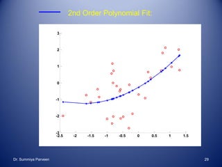
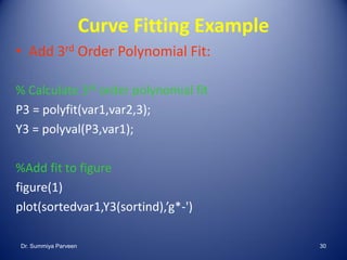
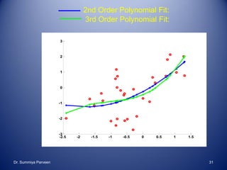
28. Curve Fitting Example
• 2nd Order Polynomial Fit:
%read data
[var1, var2] = textread(‘week8_testdata2.txt','%f%f','headerlines',1)
% Calculate 2nd order polynomial fit
P2 = polyfit(var1,var2,2);
Y2 = polyval(P2,var1);
%Plot fit
close all
figure(1)
hold on
plot(var1,var2,'ro')
[sortedvar1, sortind] = sort(var1)
plot(sortedvar1,Y2(sortind),'b*-')Dr. Summiya Parveen 28

29. 2nd Order Polynomial Fit:
-2.5 -2 -1.5 -1 -0.5 0 0.5 1 1.5
-3
-2
-1
0
1
2
3
Dr. Summiya Parveen 29

30. Curve Fitting Example
• Add 3rd Order Polynomial Fit:
% Calculate 3rd order polynomial fit
P3 = polyfit(var1,var2,3);
Y3 = polyval(P3,var1);
%Add fit to figure
figure(1)
plot(sortedvar1,Y3(sortind),’g*-')
Dr. Summiya Parveen 30

31. -2.5 -2 -1.5 -1 -0.5 0 0.5 1 1.5
-3
-2
-1
0
1
2
3
2nd Order Polynomial Fit:
3rd Order Polynomial Fit:
Dr. Summiya Parveen 31

32. Curve Fitting Example
• Add 4th Order Polynomial Fit:
% Calculate 4th order polynomial fit
P4 = polyfit(var1,var2,4);
Y4 = polyval(P4,var1);
%Add fit to figure
figure(1)
plot(sortedvar1,Y4(sortind),’k*-')
Dr. Summiya Parveen 32

33. -2.5 -2 -1.5 -1 -0.5 0 0.5 1 1.5
-3
-2
-1
0
1
2
3
2nd Order Polynomial Fit:
3rd Order Polynomial Fit:
4th Order Polynomial Fit:
Dr. Summiya Parveen 33

34. -2.5 -2 -1.5 -1 -0.5 0 0.5 1 1.5
-3
-2
-1
0
1
2
3
Assessing Goodness of Fit
Example Solution
% recall var1 contains x values and var2 contains y values of data points
ypred = polyval(P2,var1);
dev = var2 - mean(2);
SST = sum(dev.^2);
resid = var2 - ypred;
SSE = sum(resid.^2);
normr = sqrt(SSE); % residual norm
Rsq = 1 - SSE/SST; % R2 Error
Normr = 5.7436
Rsq = 0.8533
• The residual norm and R2 error indicate goodness of fit
2nd Order Polynomial Fit:
Dr. Summiya Parveen 34

35. Limitations of Polyfit
• Only finds a least squares best polynomial
function fit
• Cannot be used to interpolate curves or fit other
standard functions
• Requires several lines of code and the polyval()
function
Dr. Summiya Parveen 35

36. THANK YOU
Dr. Summiya Parveen 36