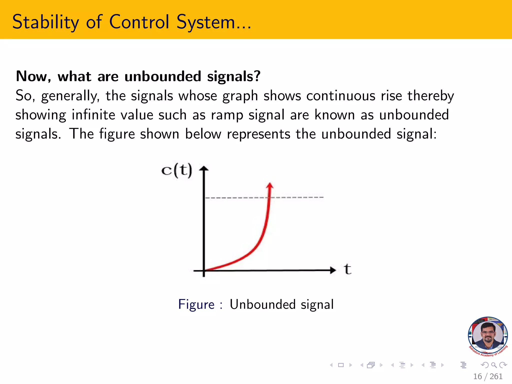
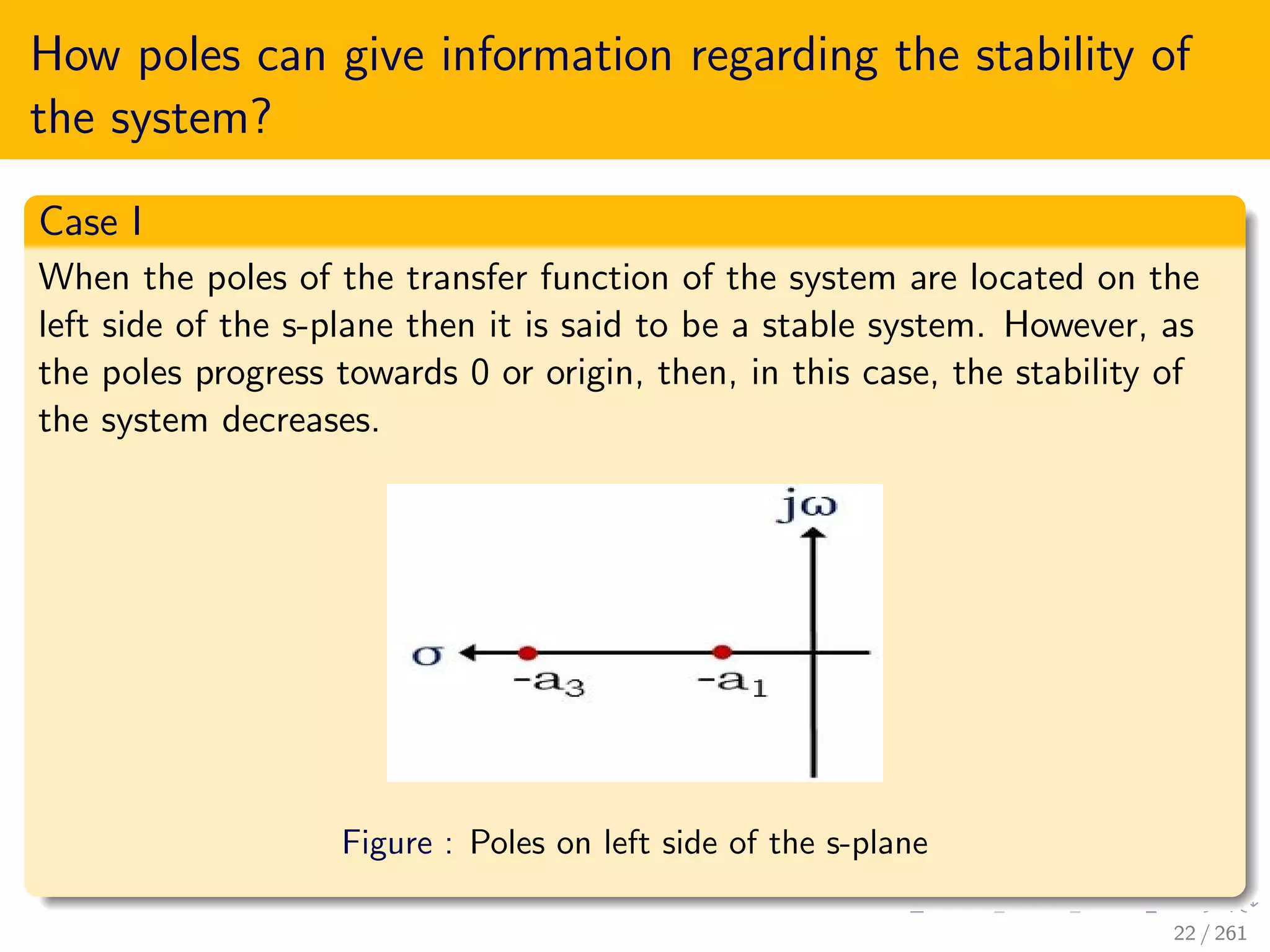
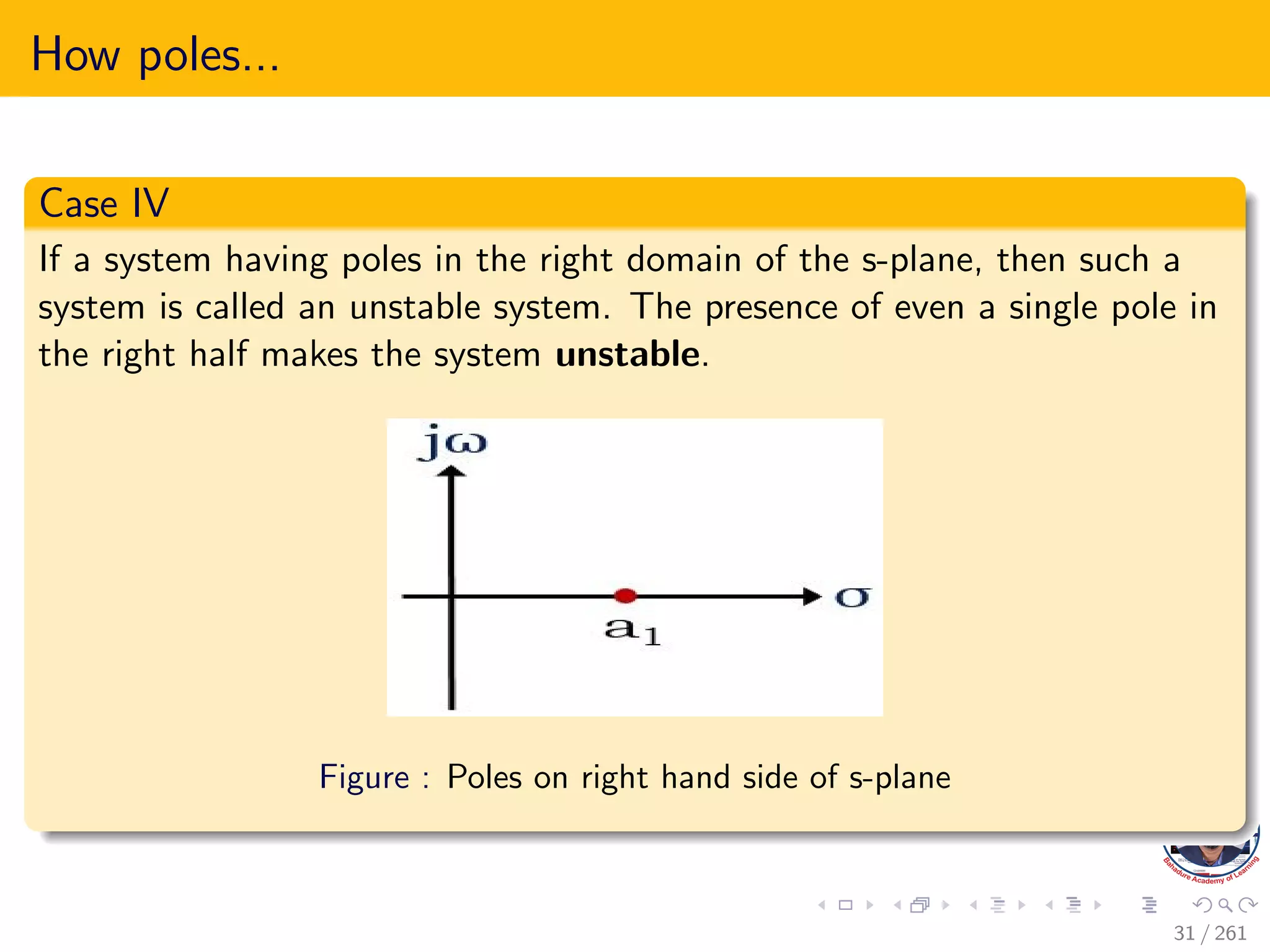
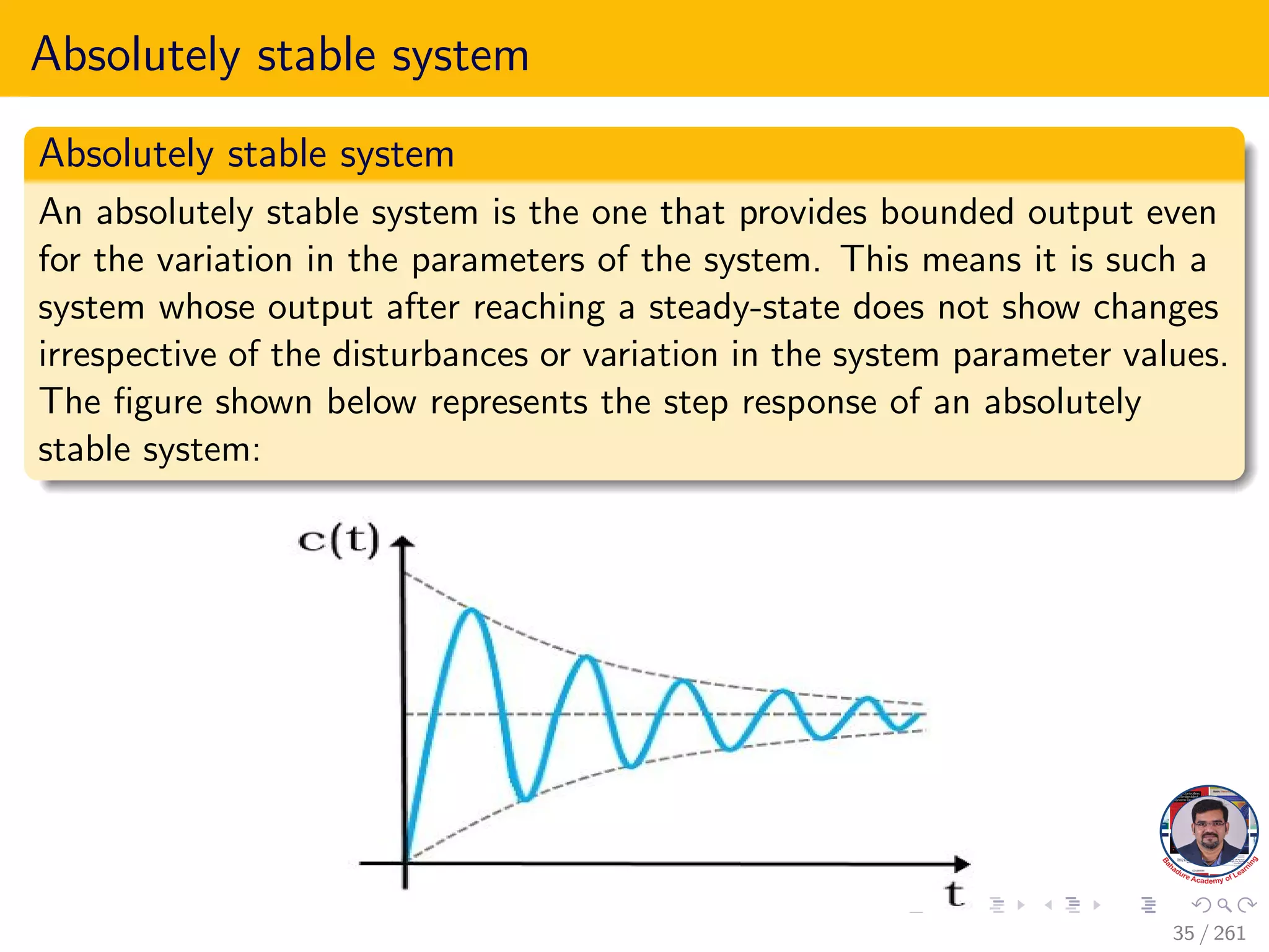
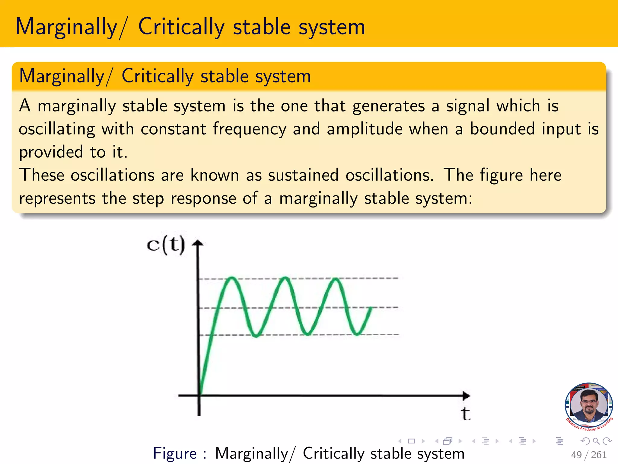
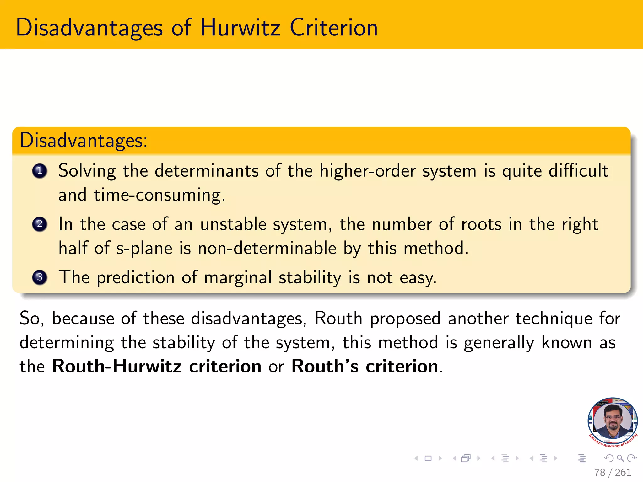
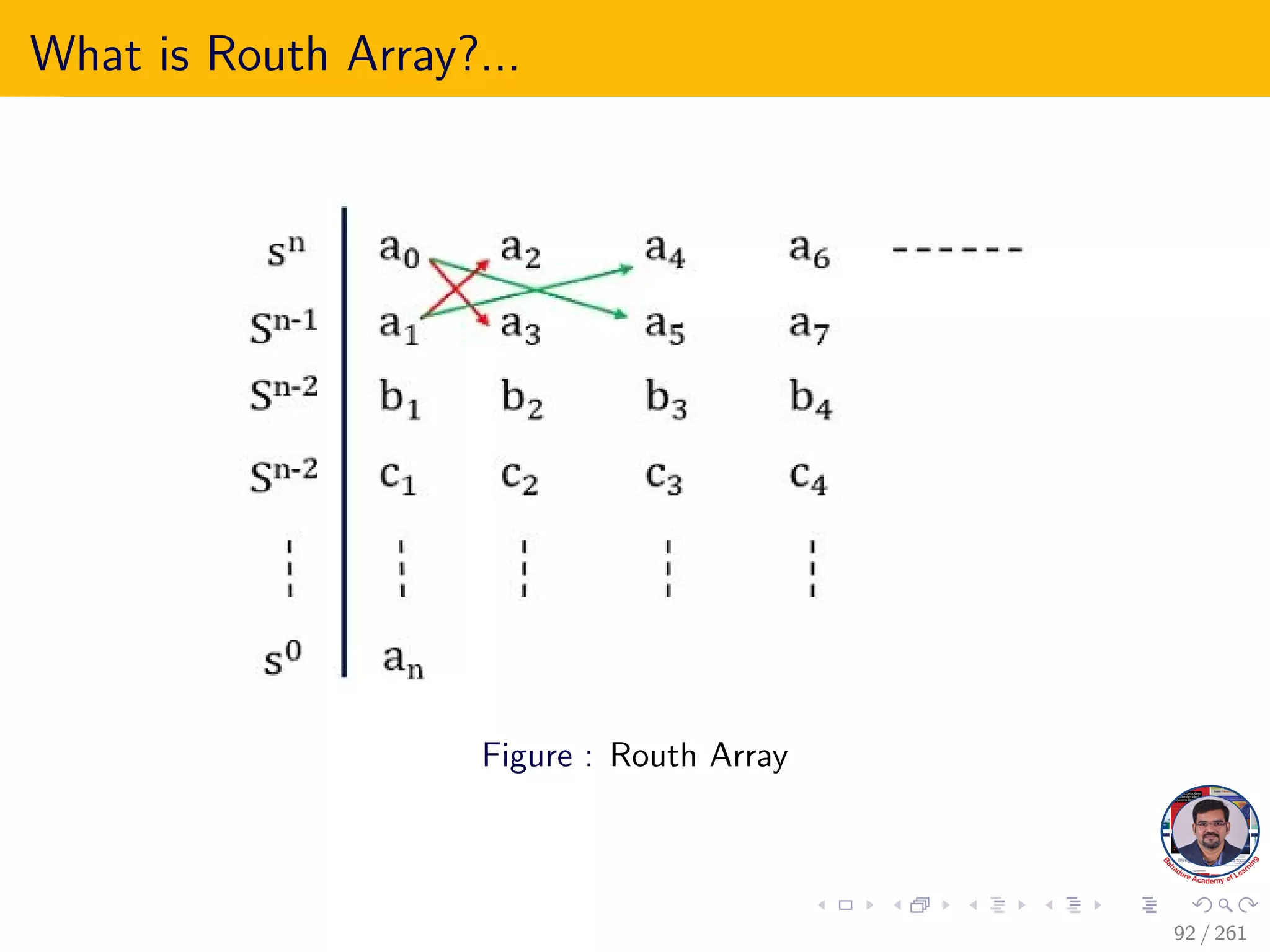
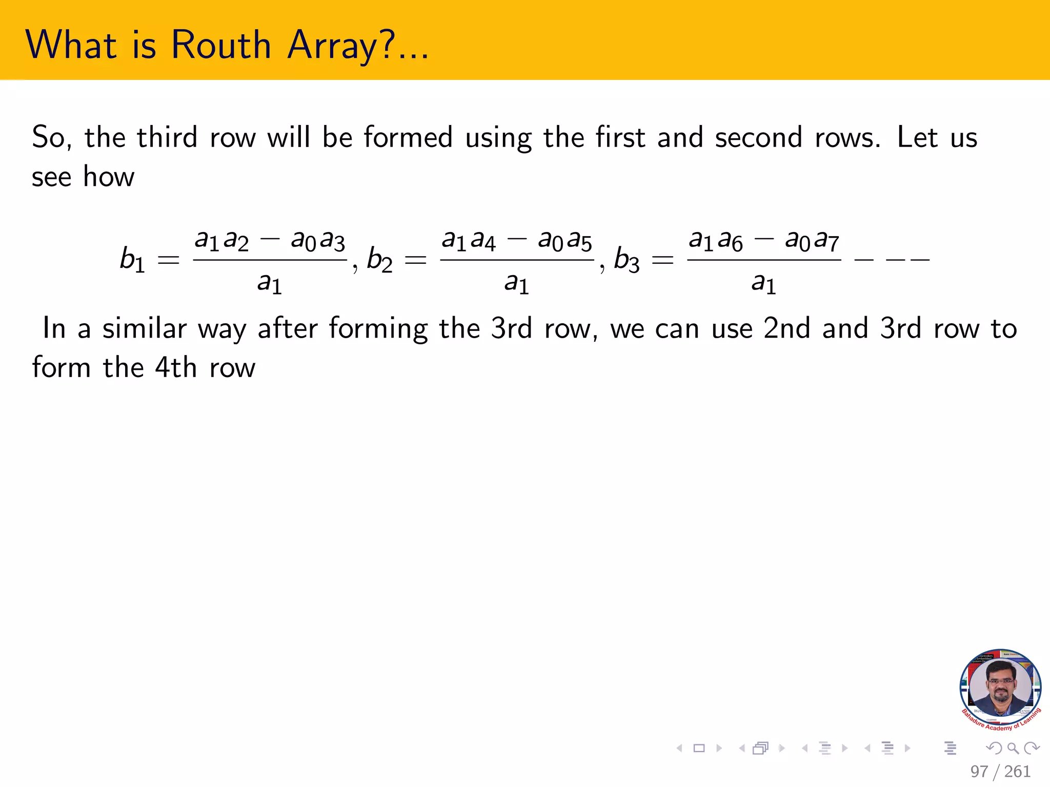
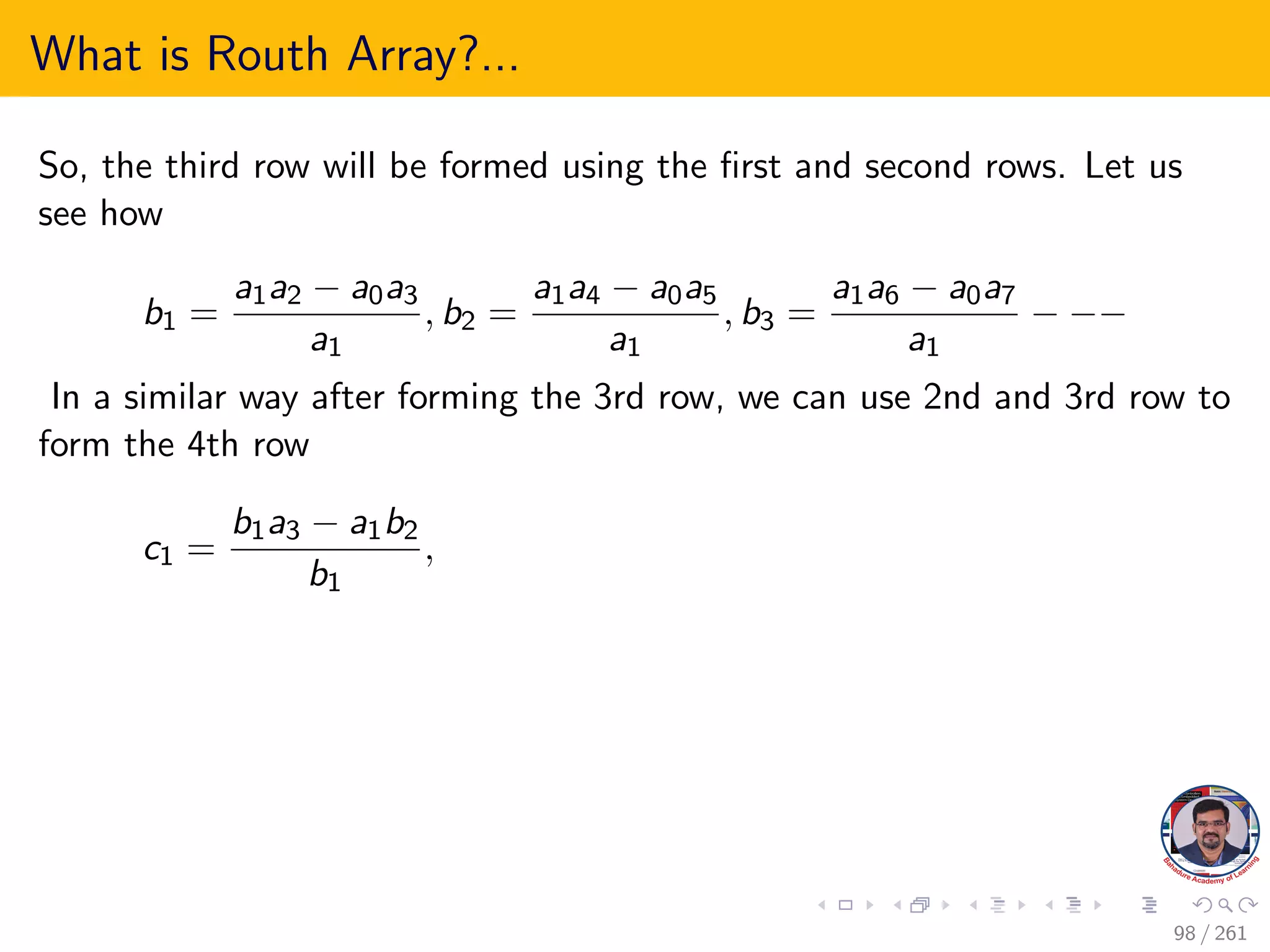
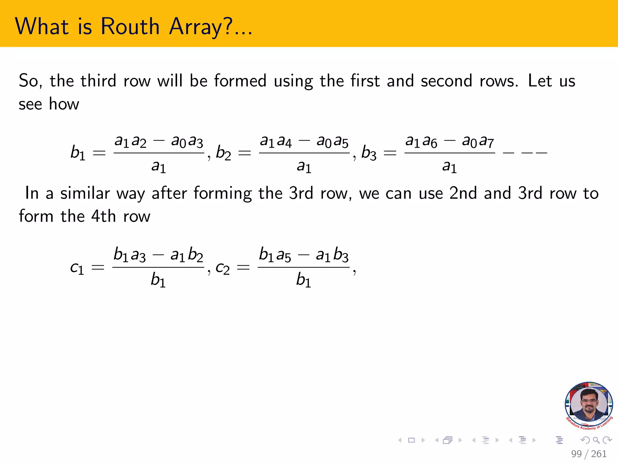
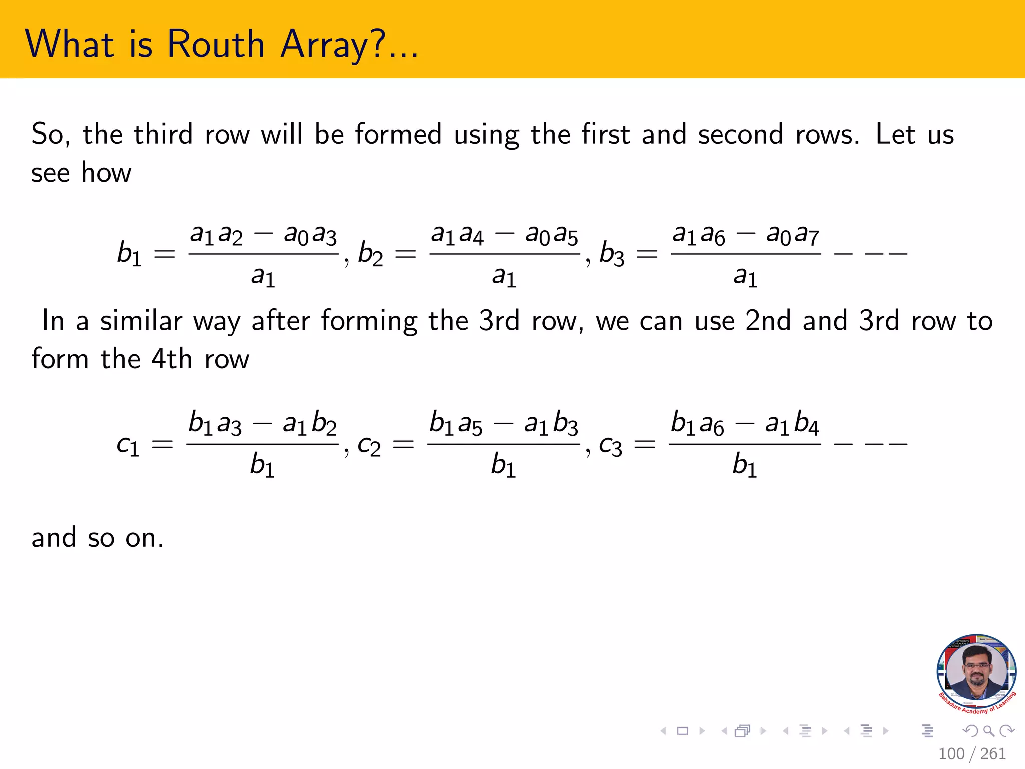
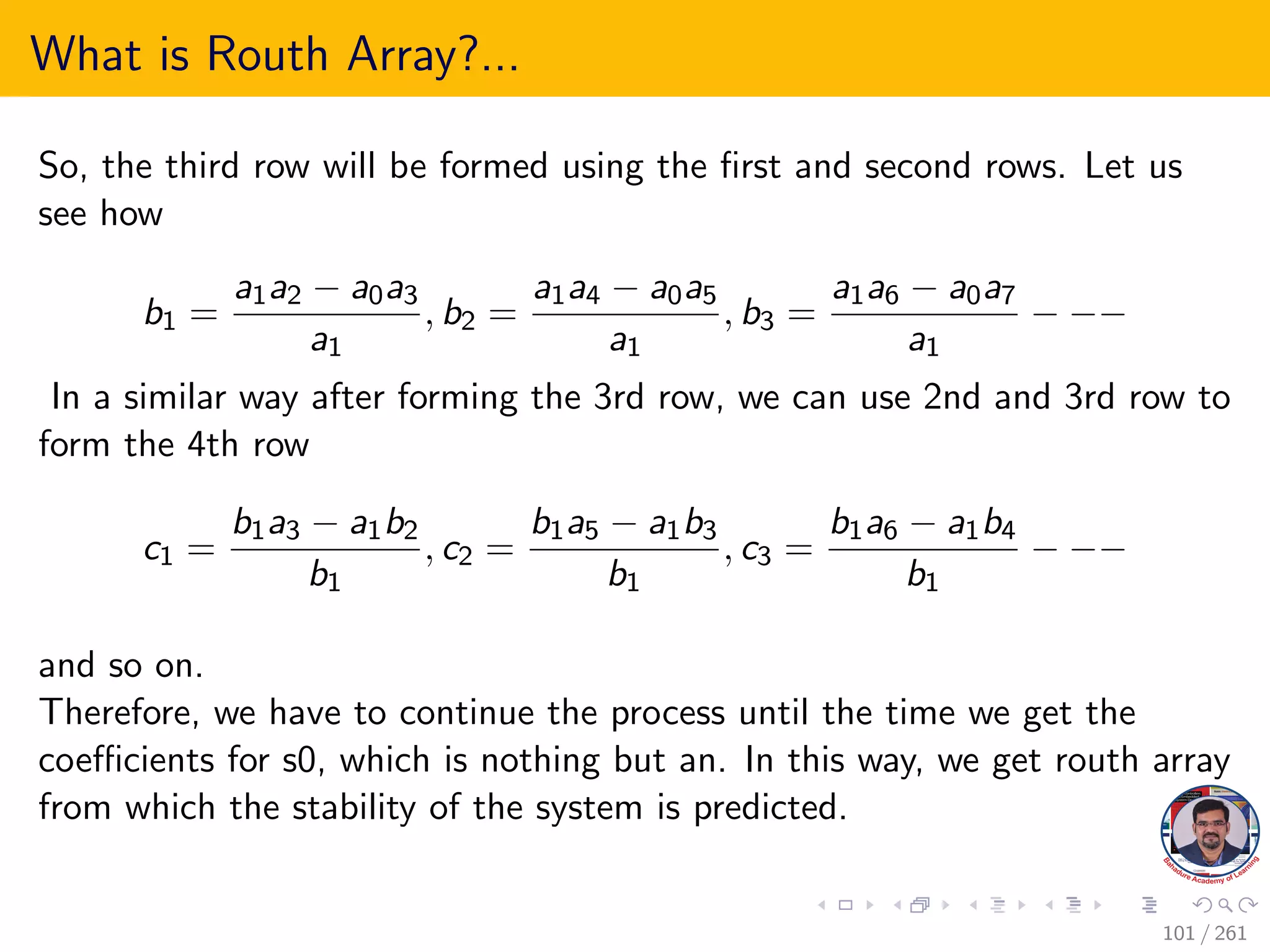
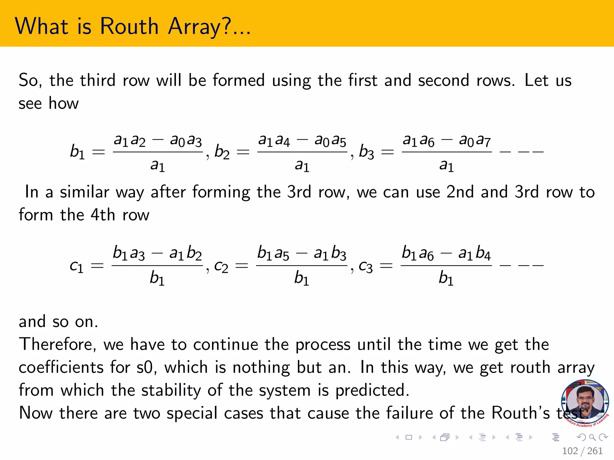
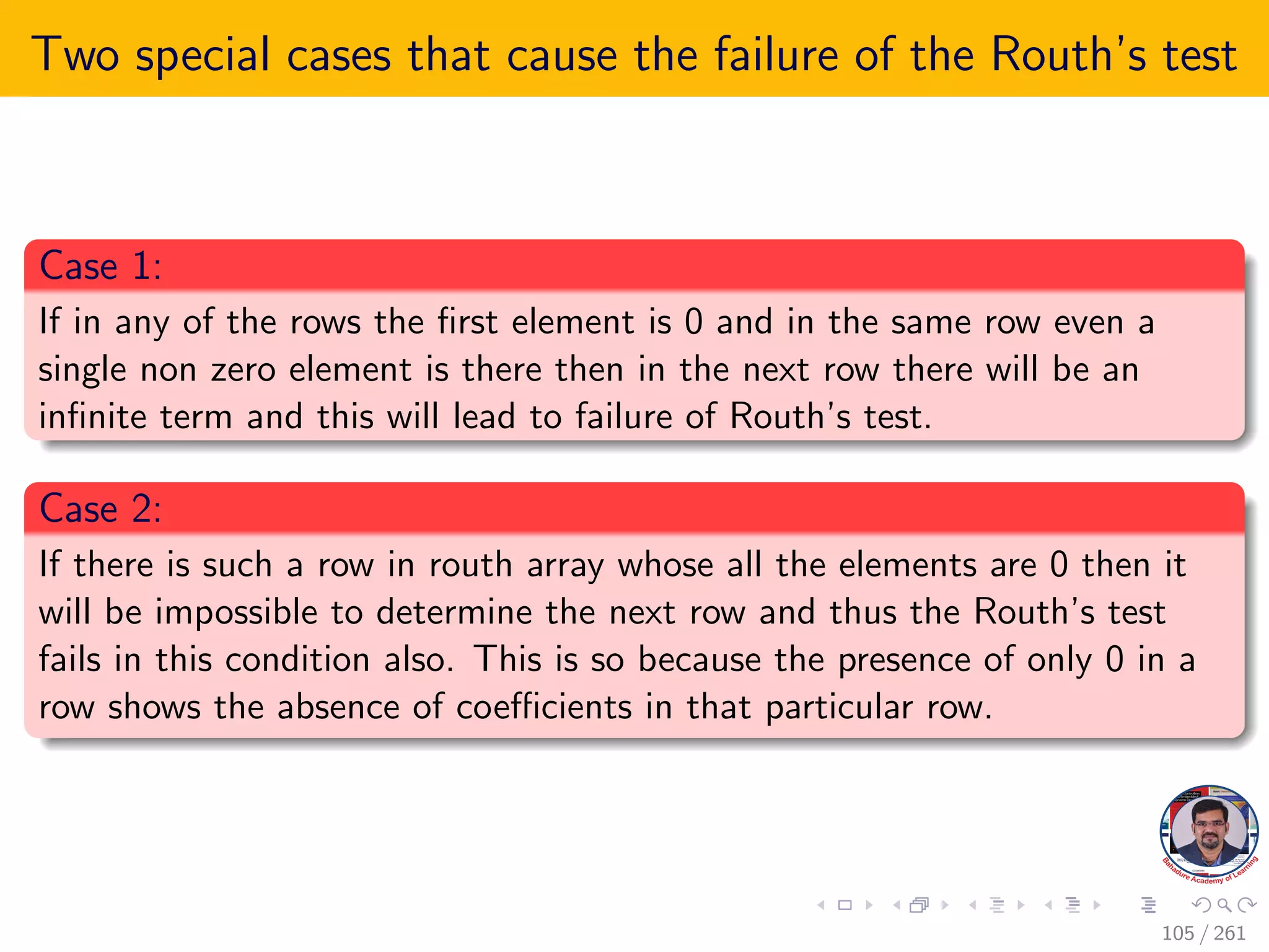
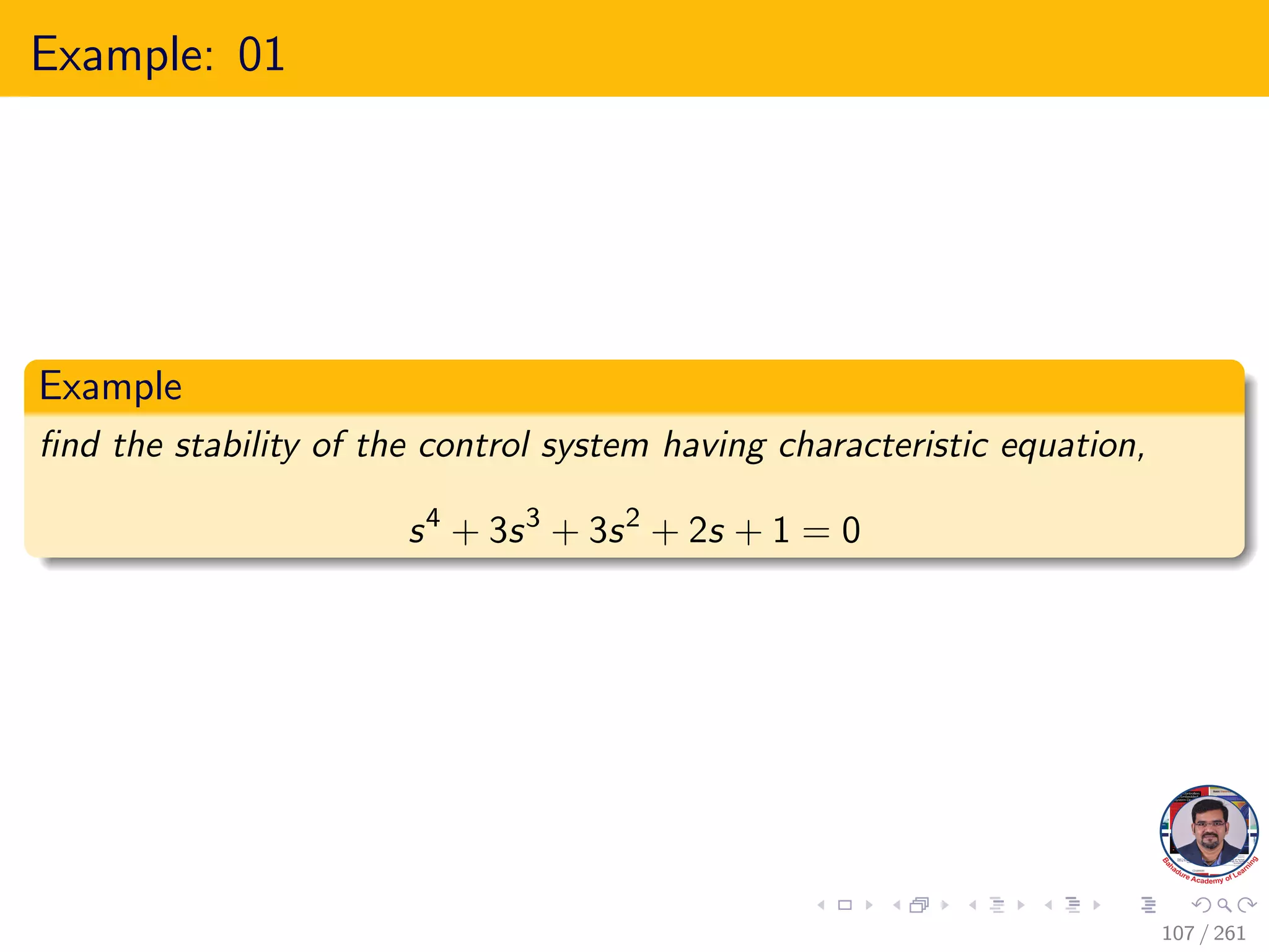
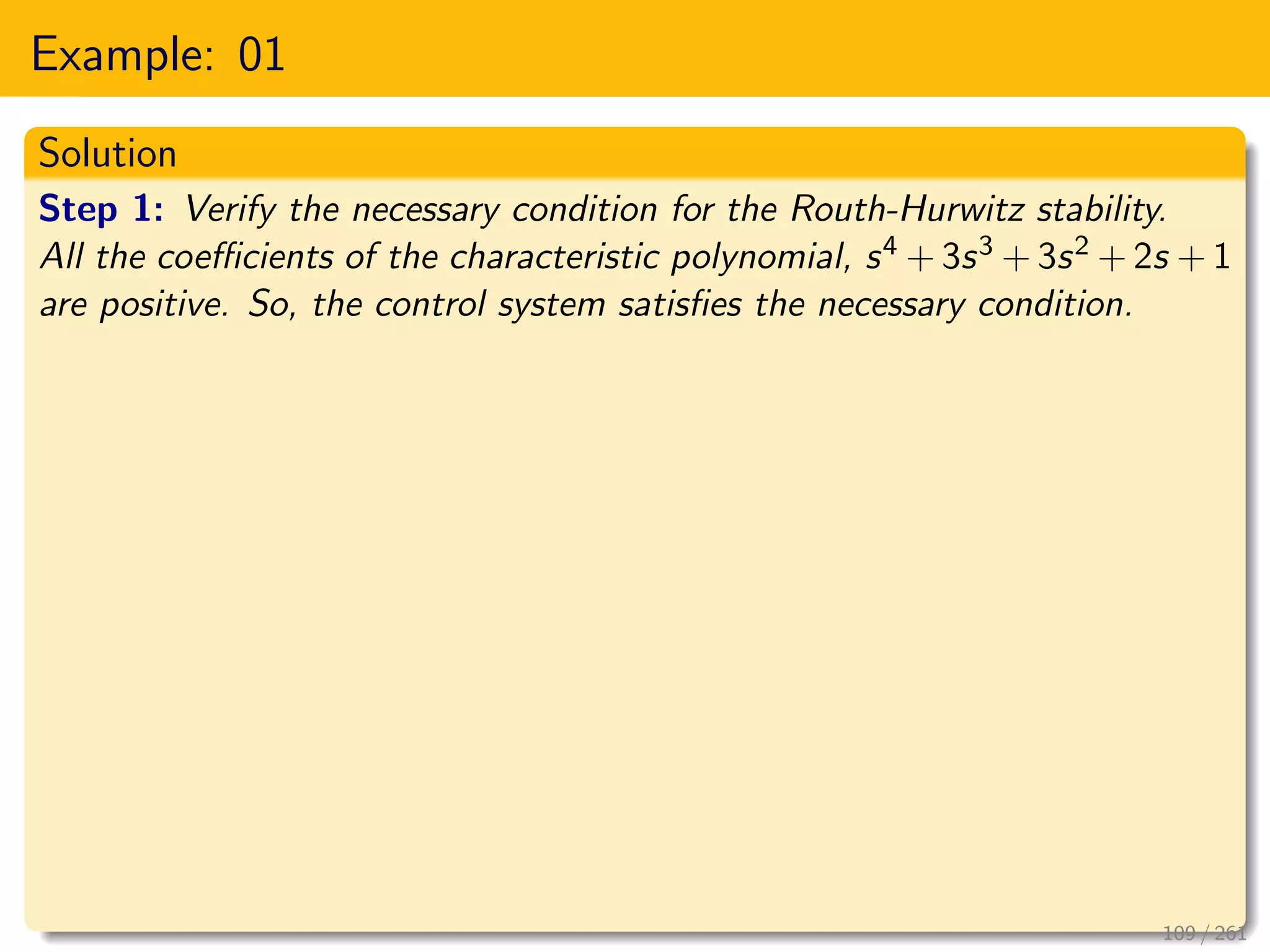
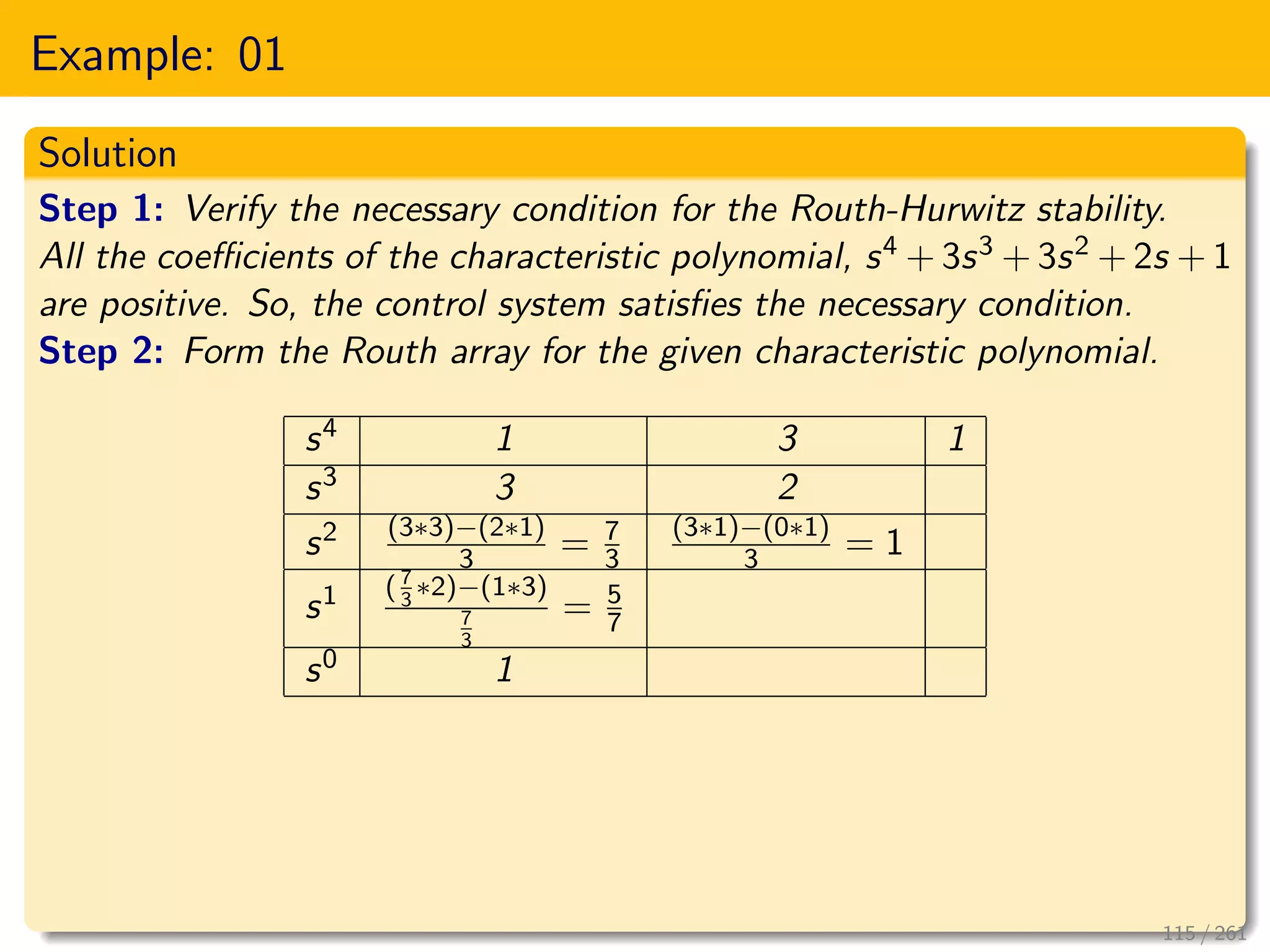
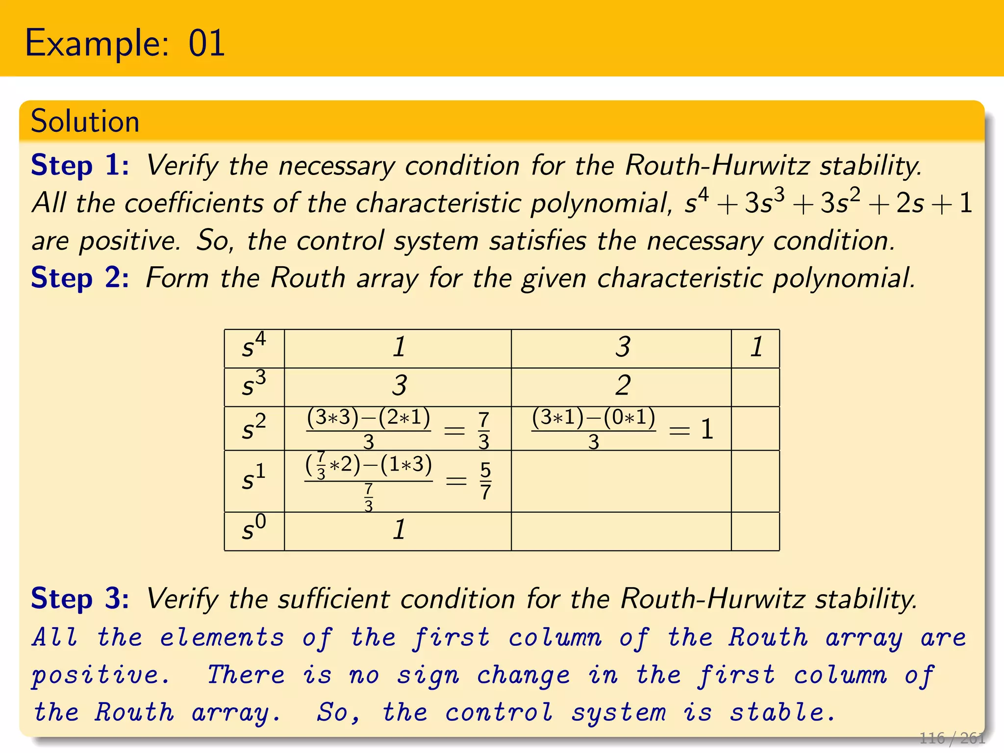
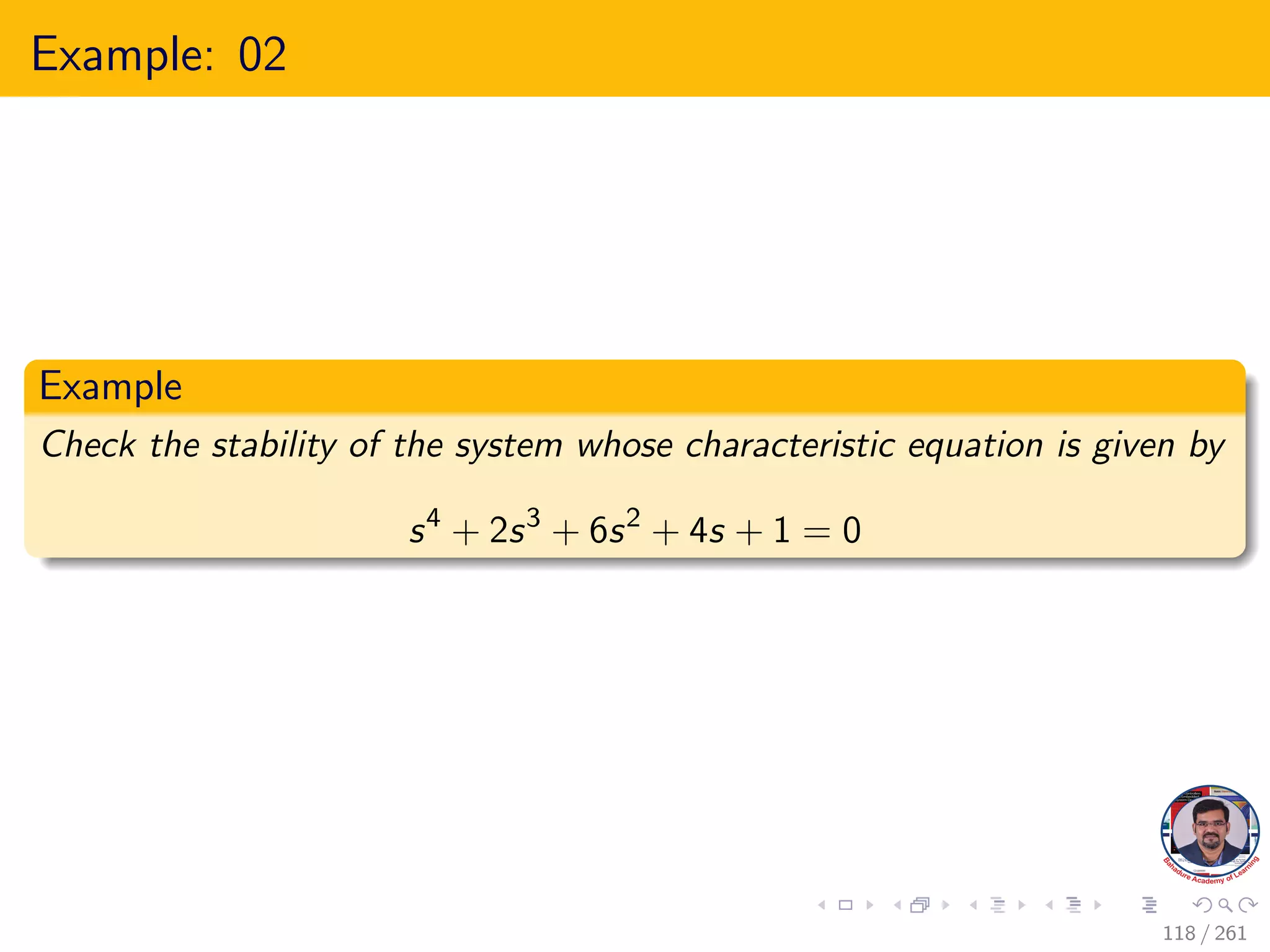
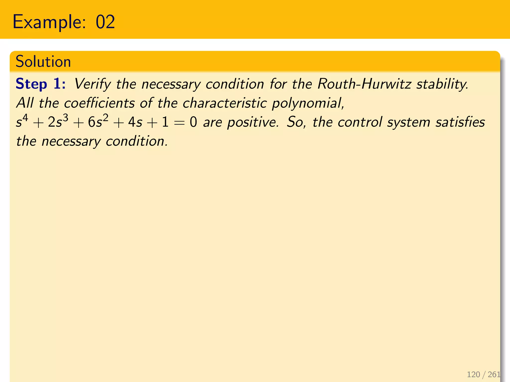
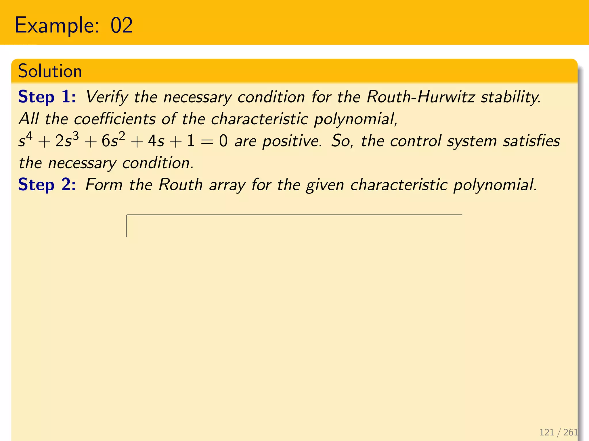
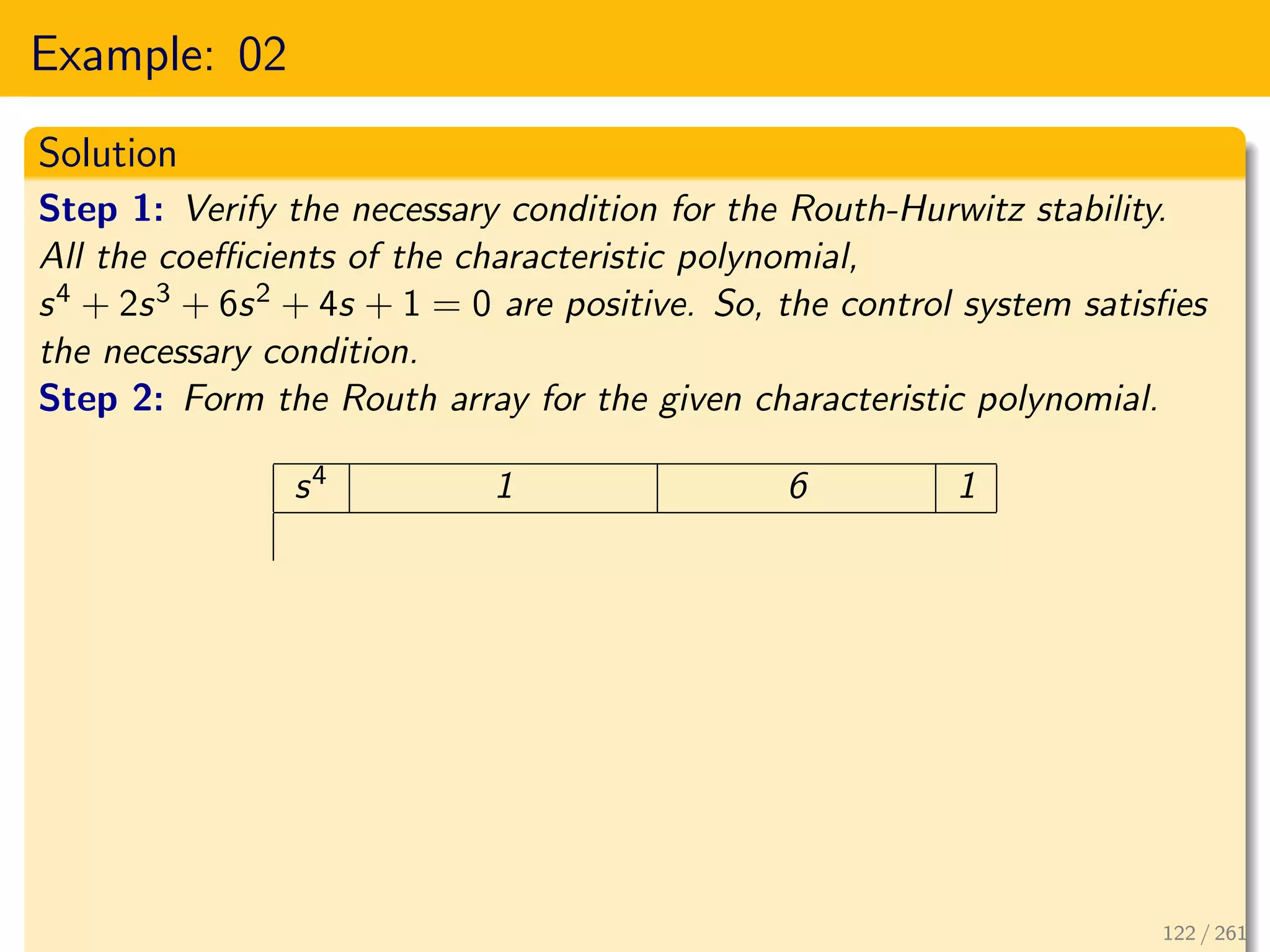
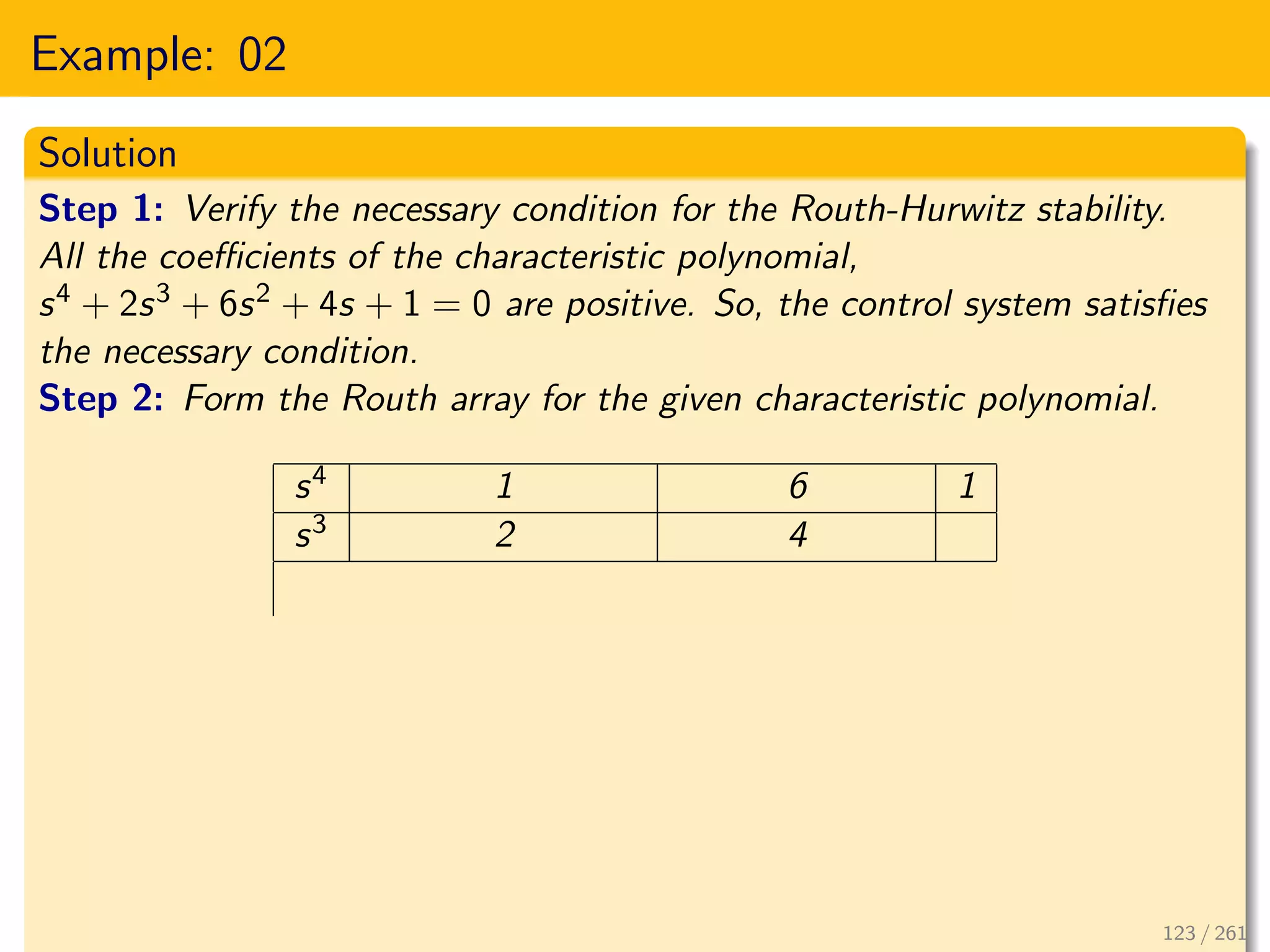
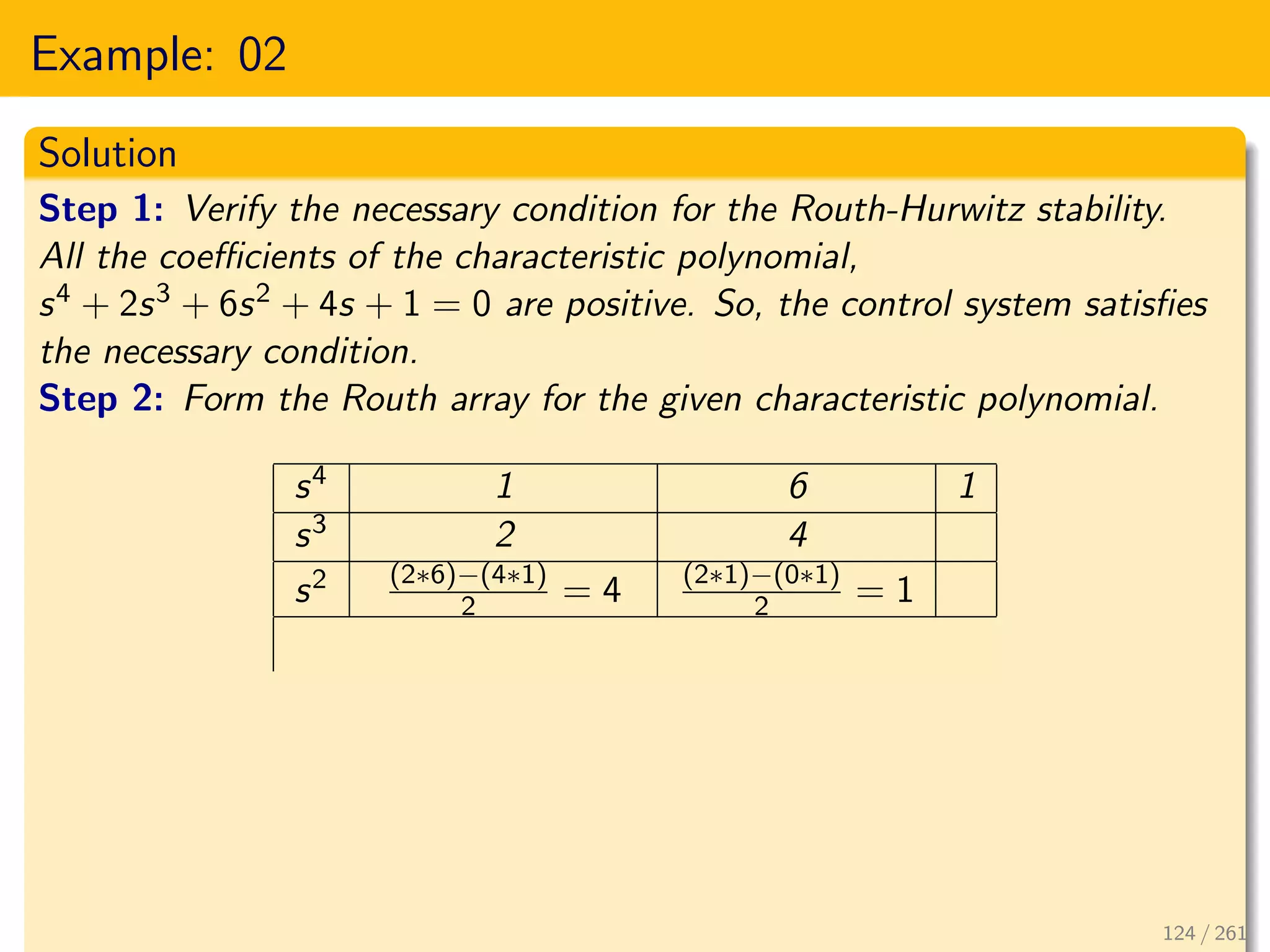
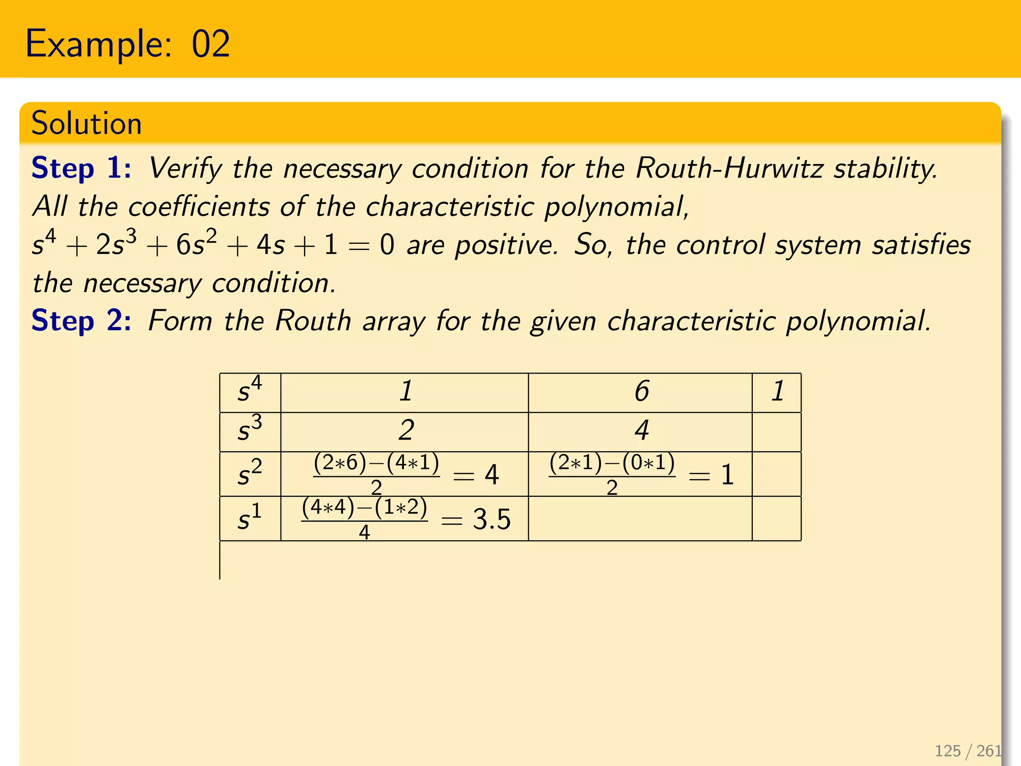
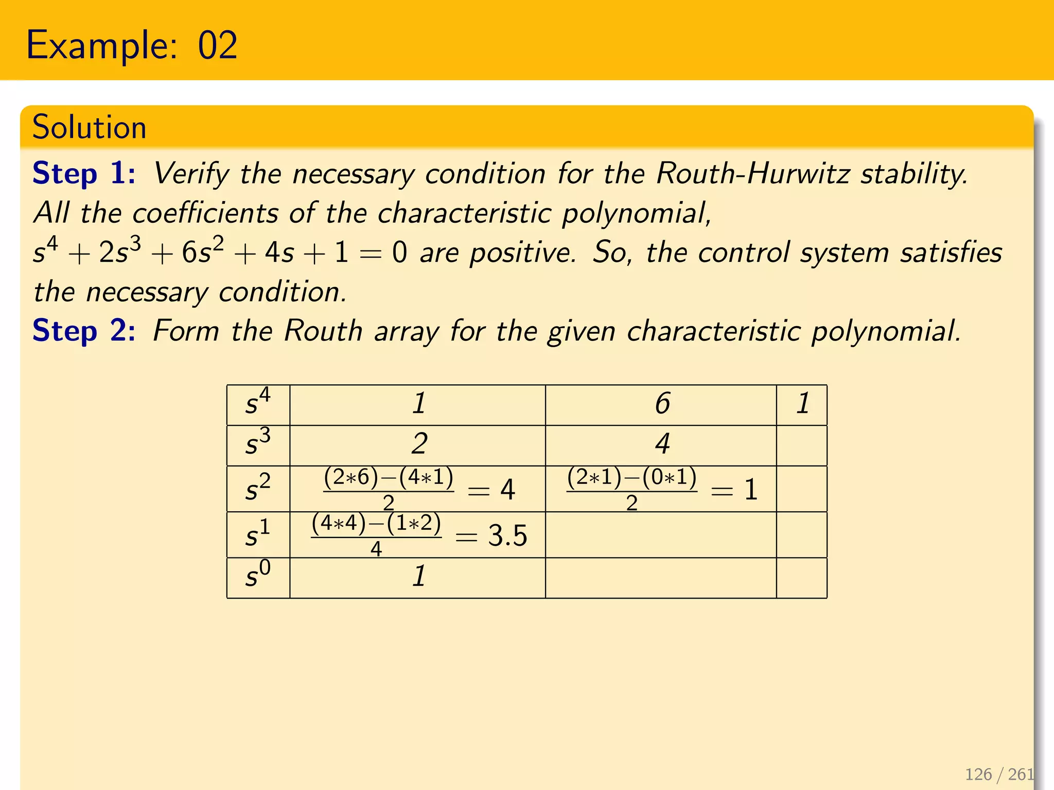
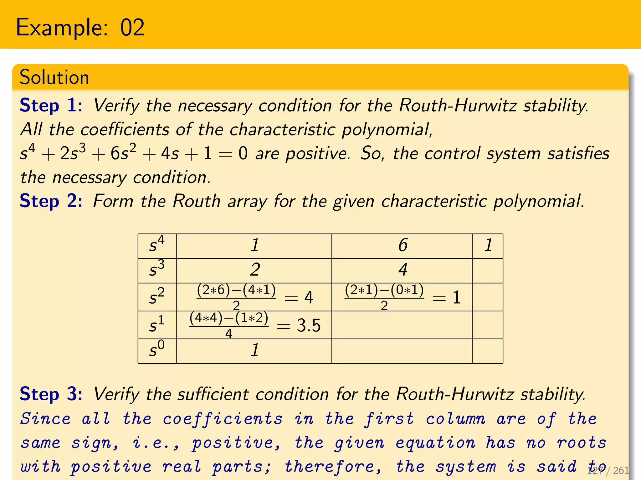
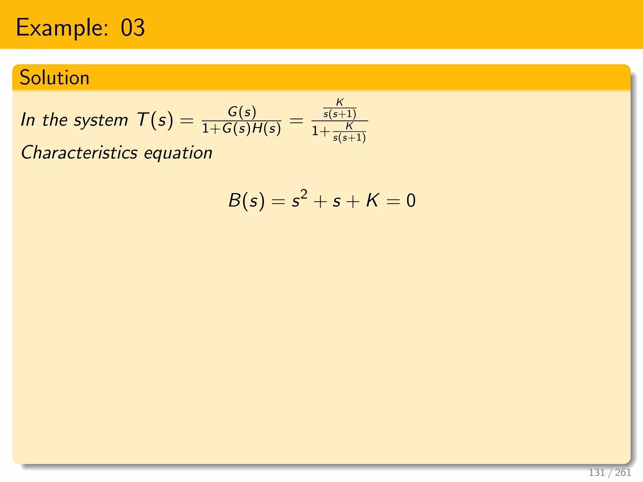
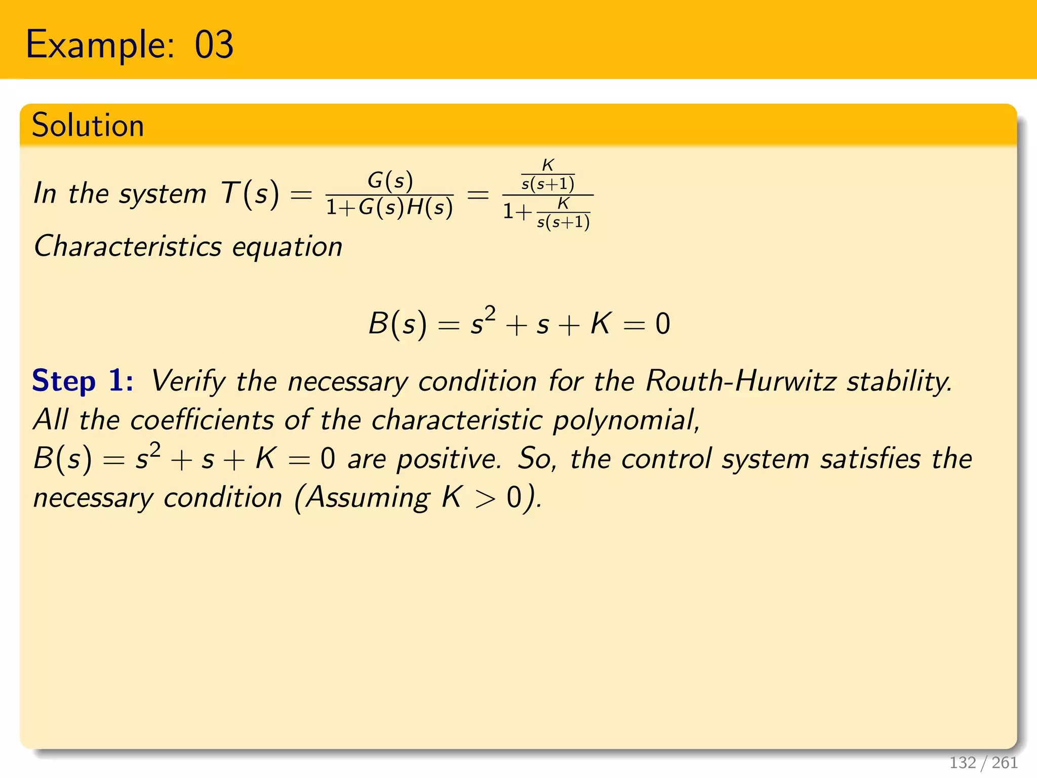
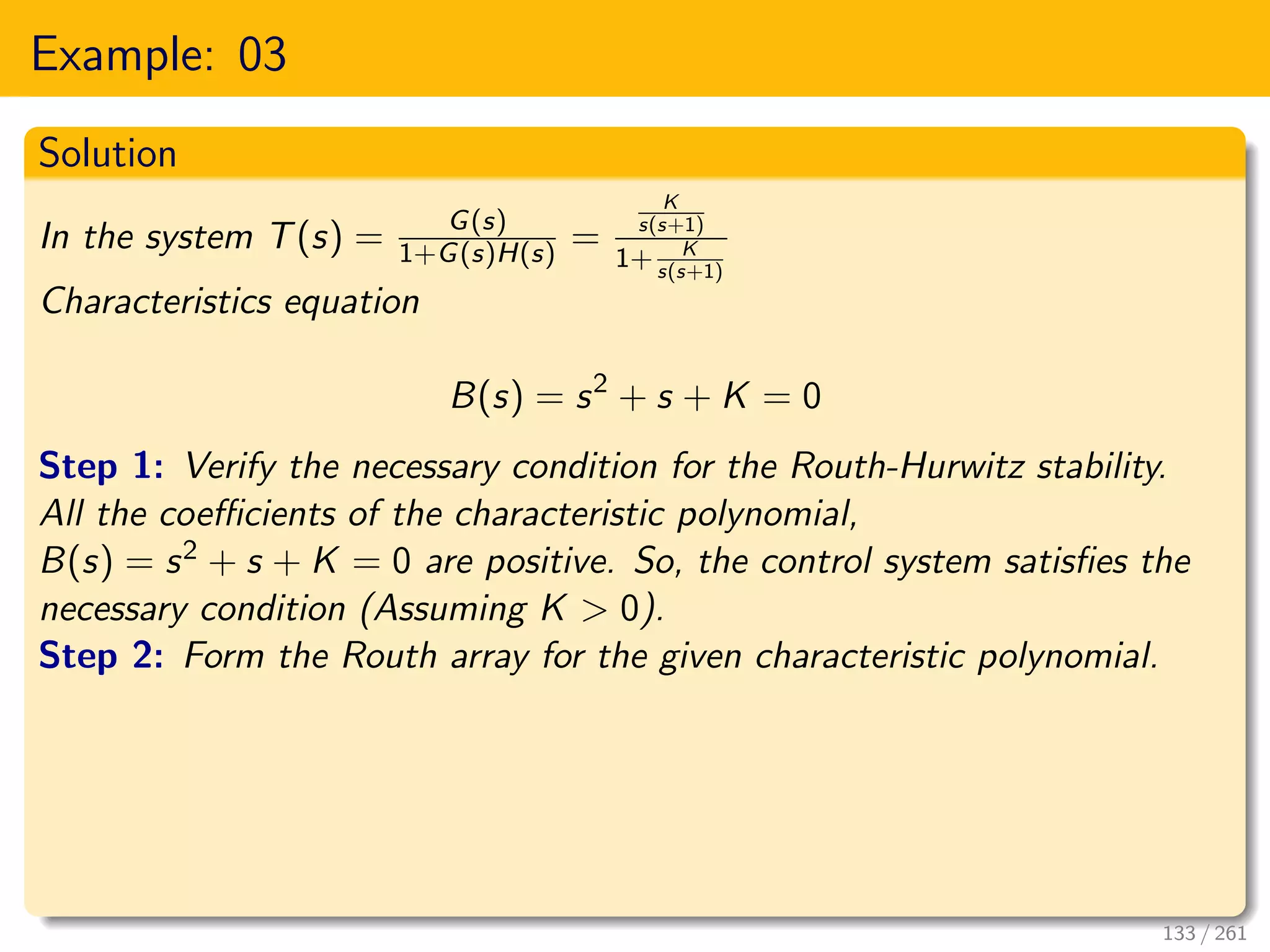
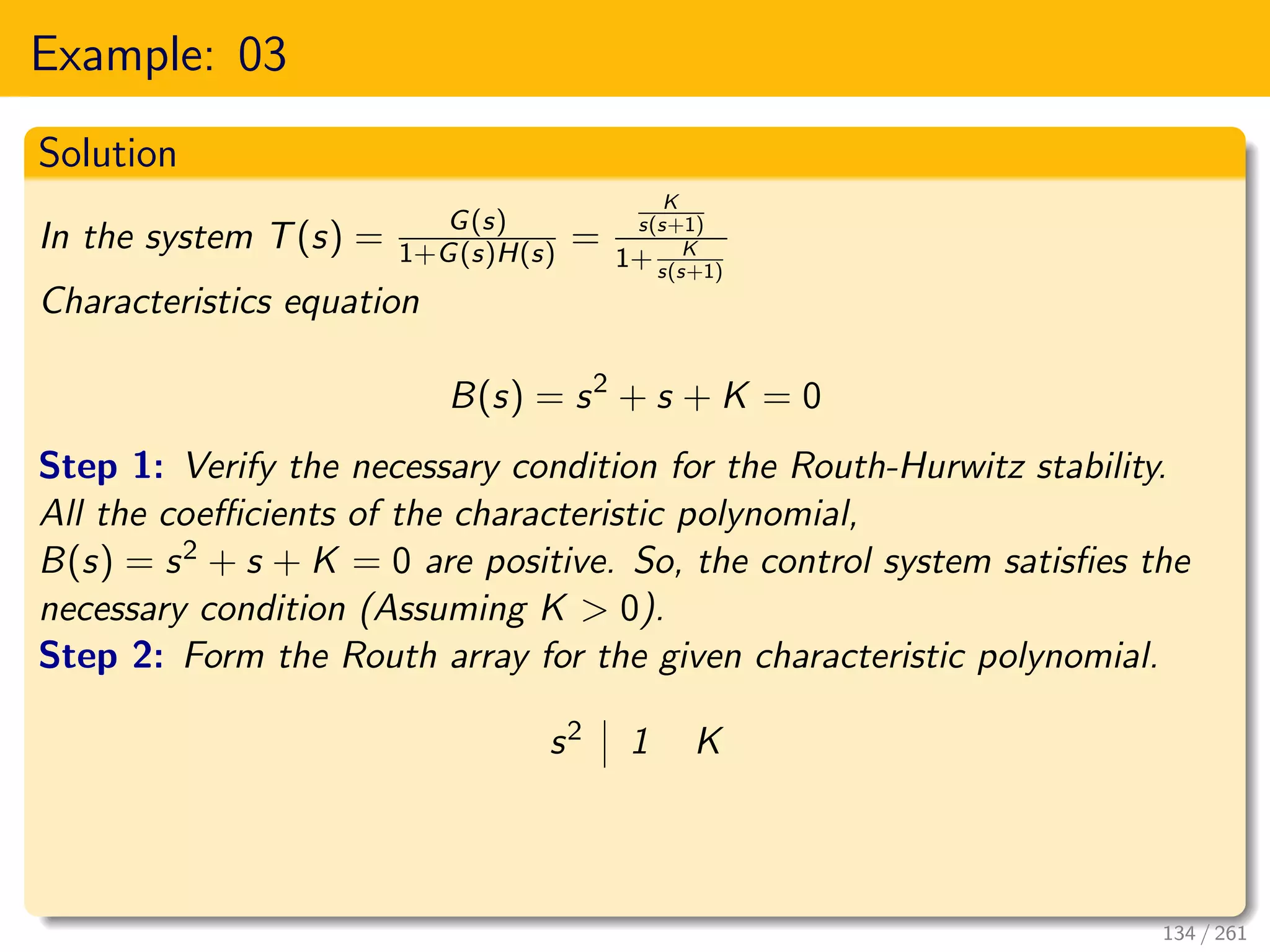
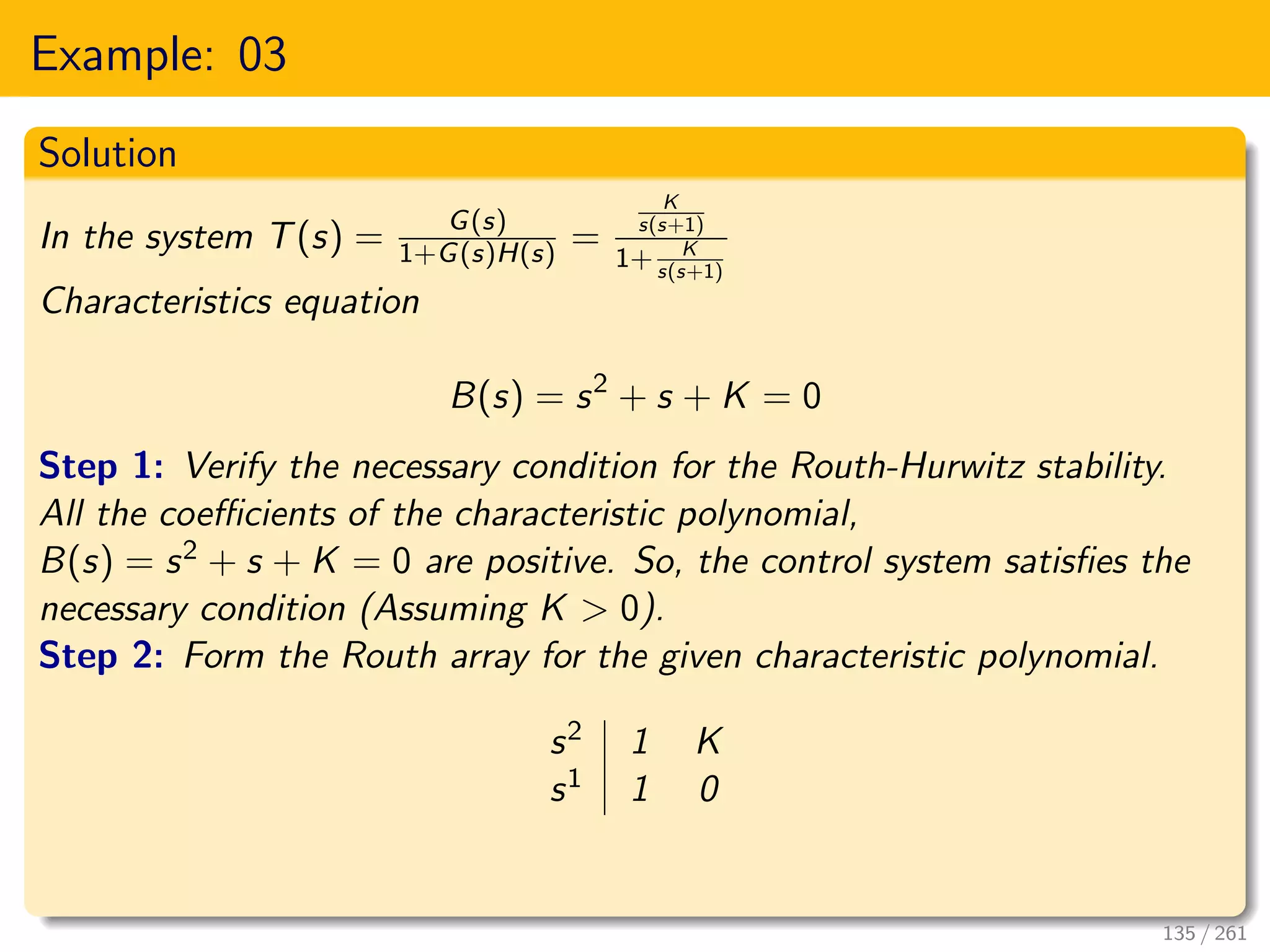
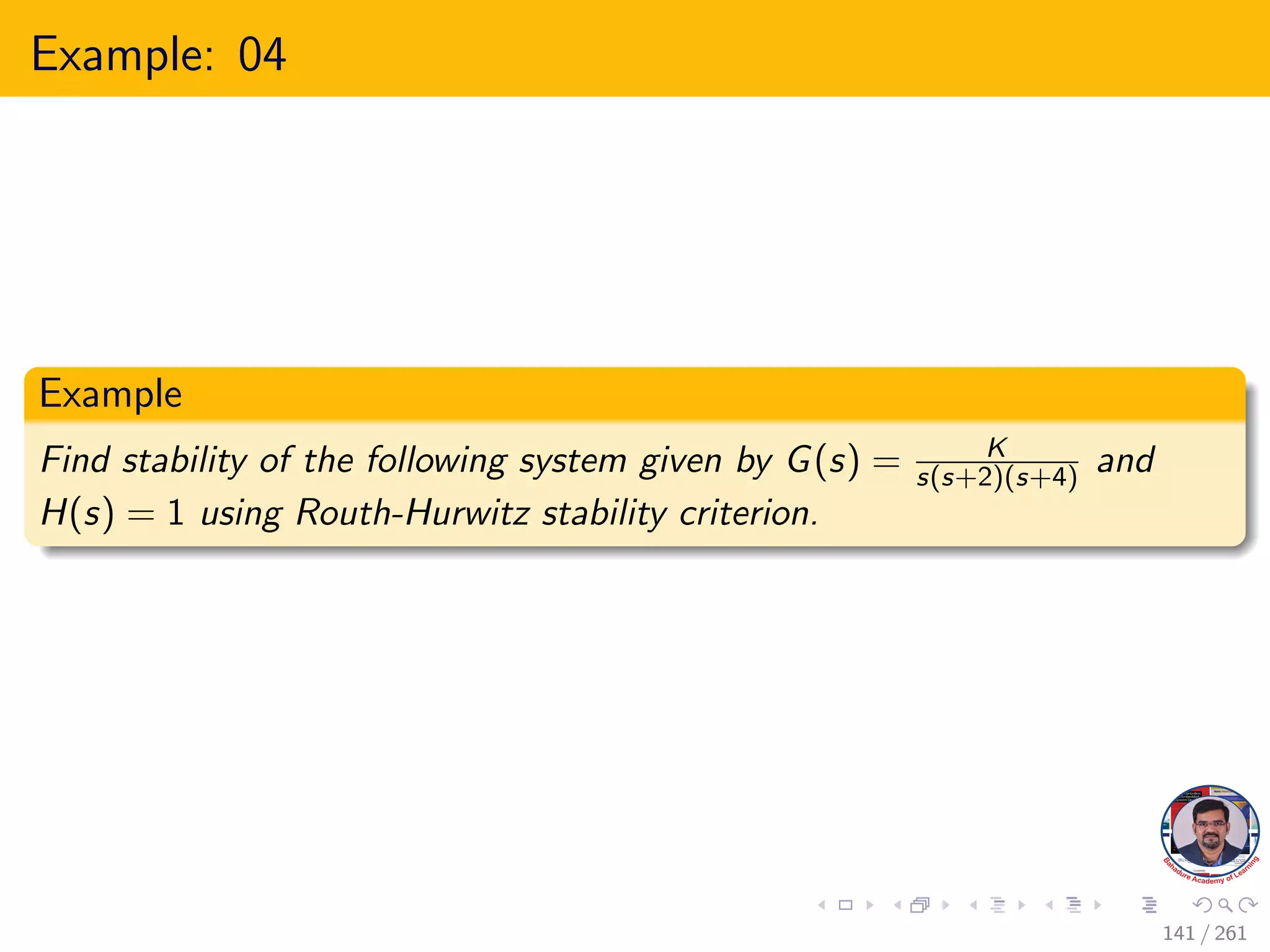
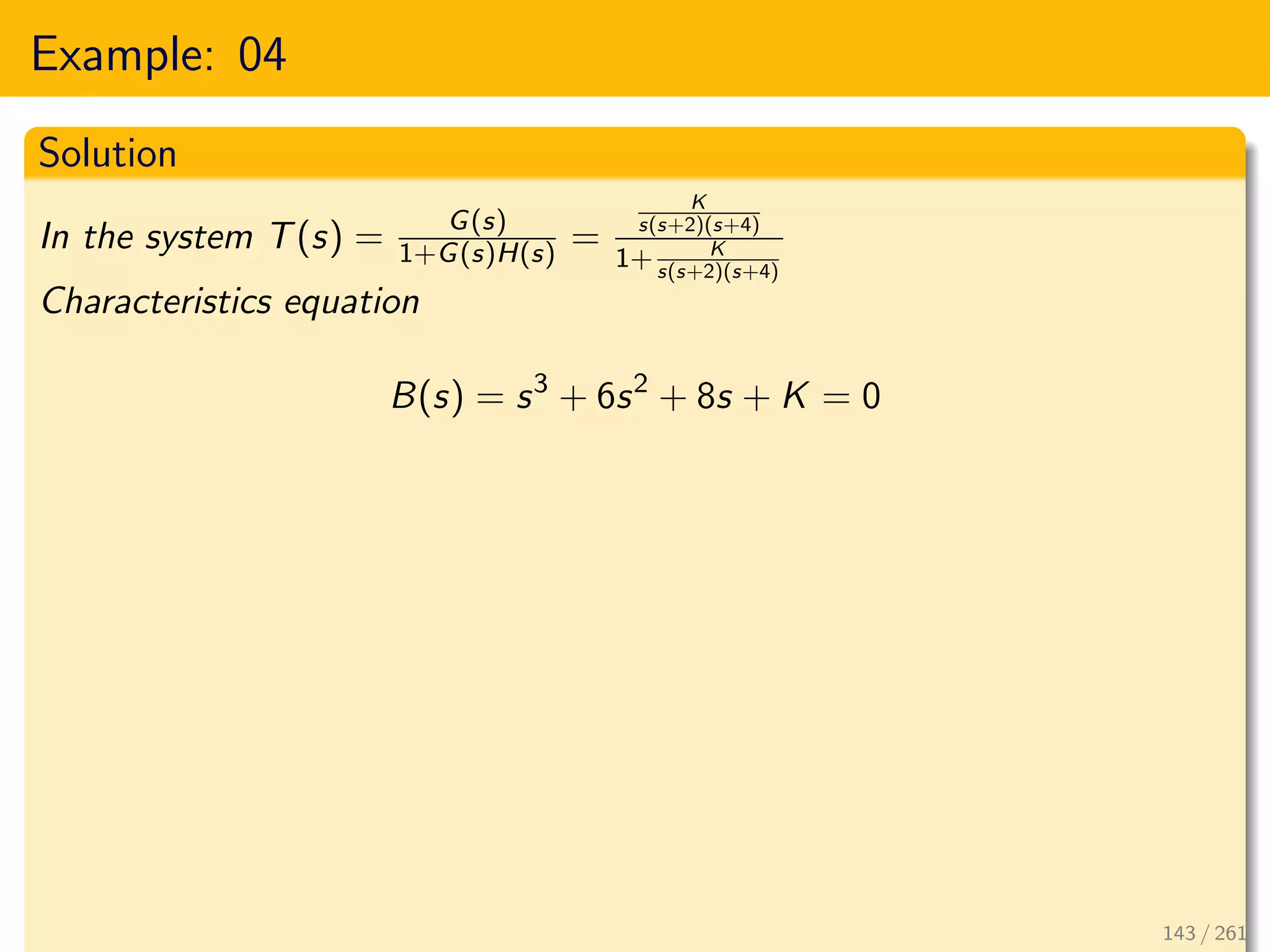
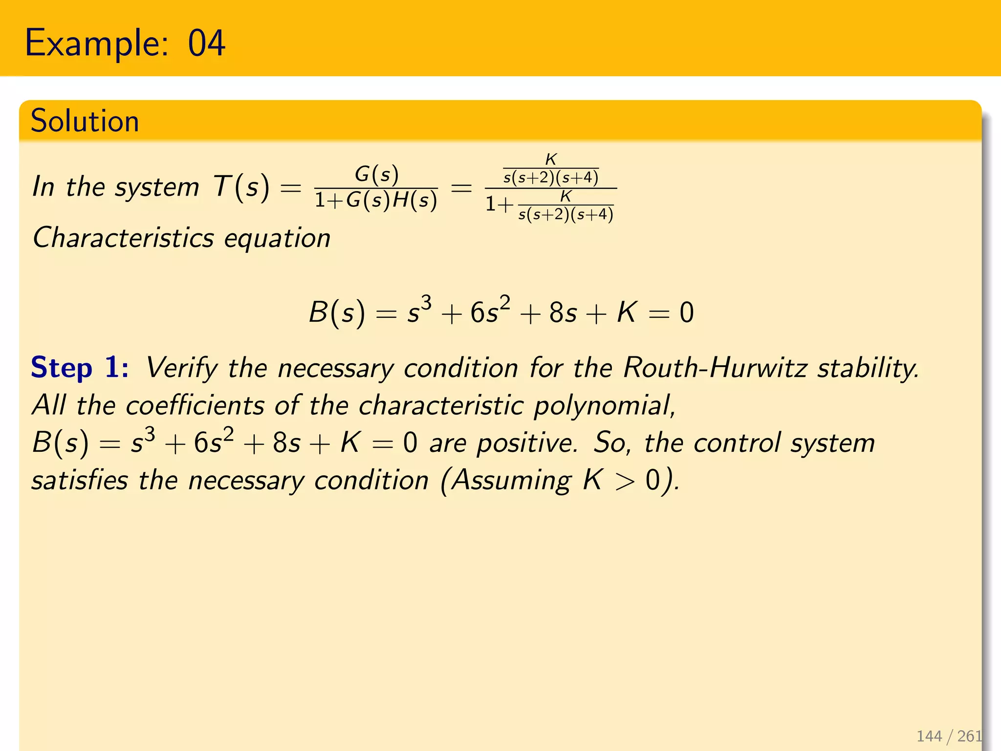
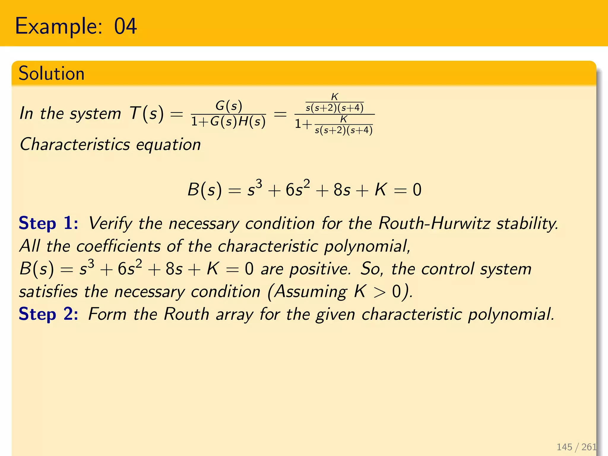
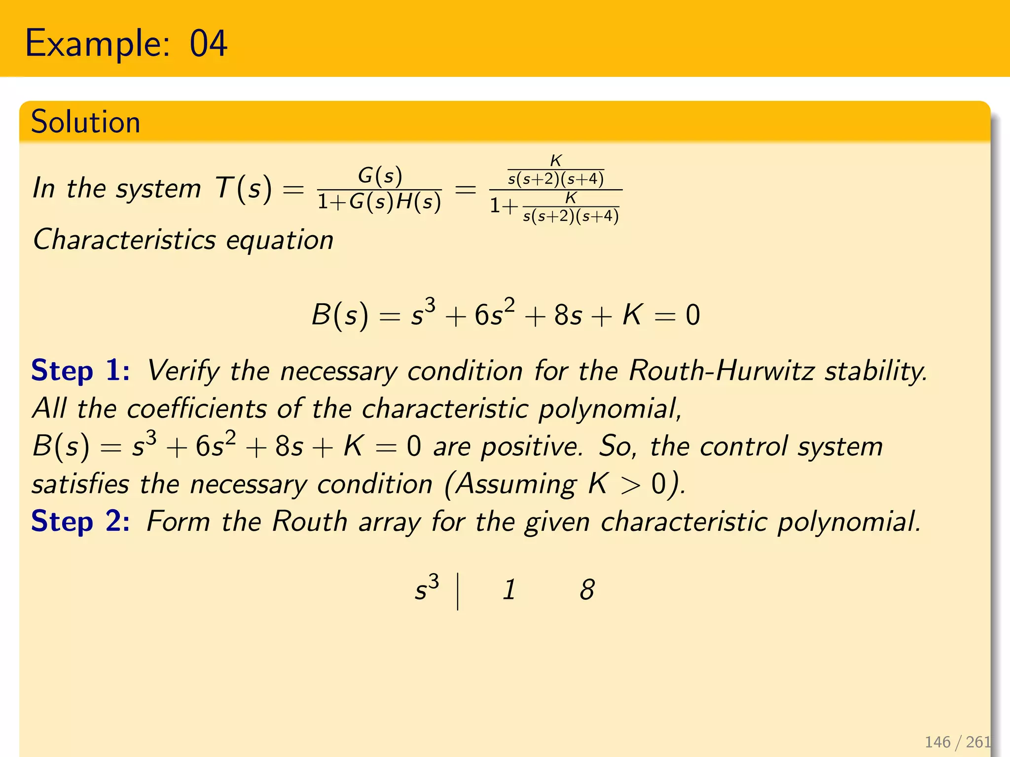
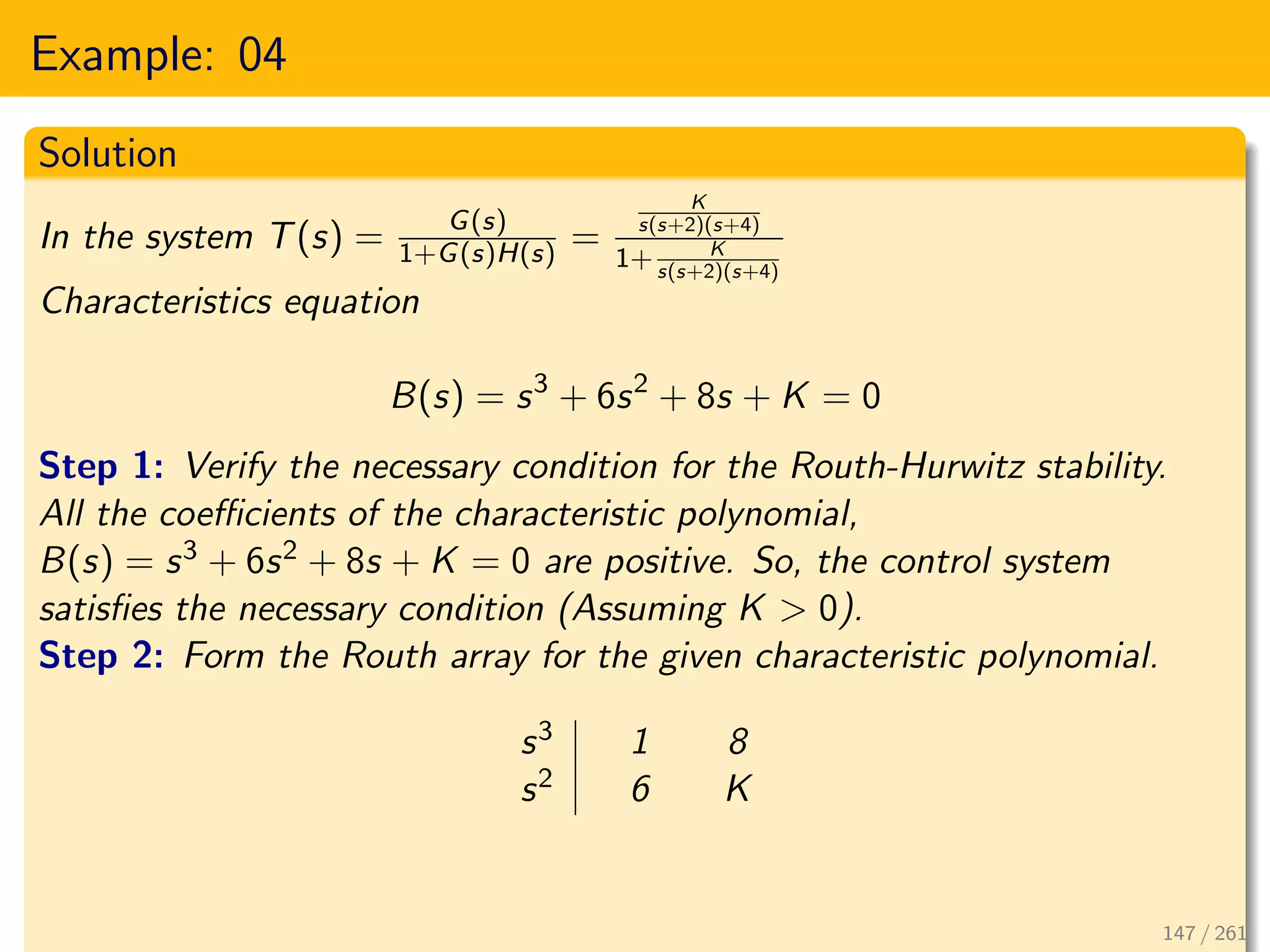
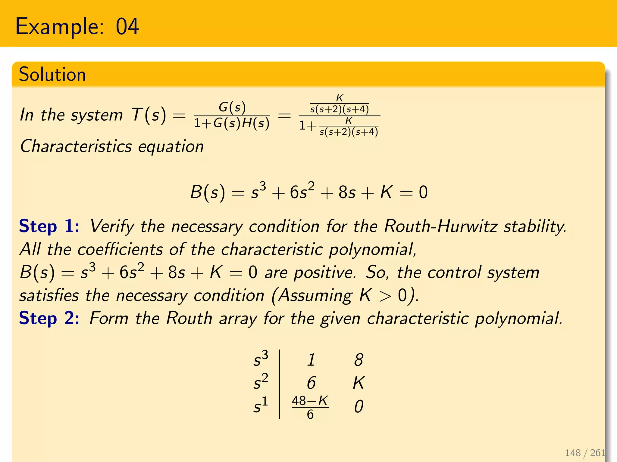
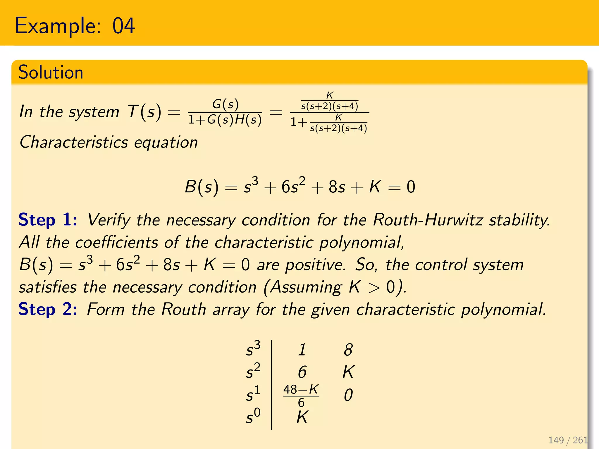
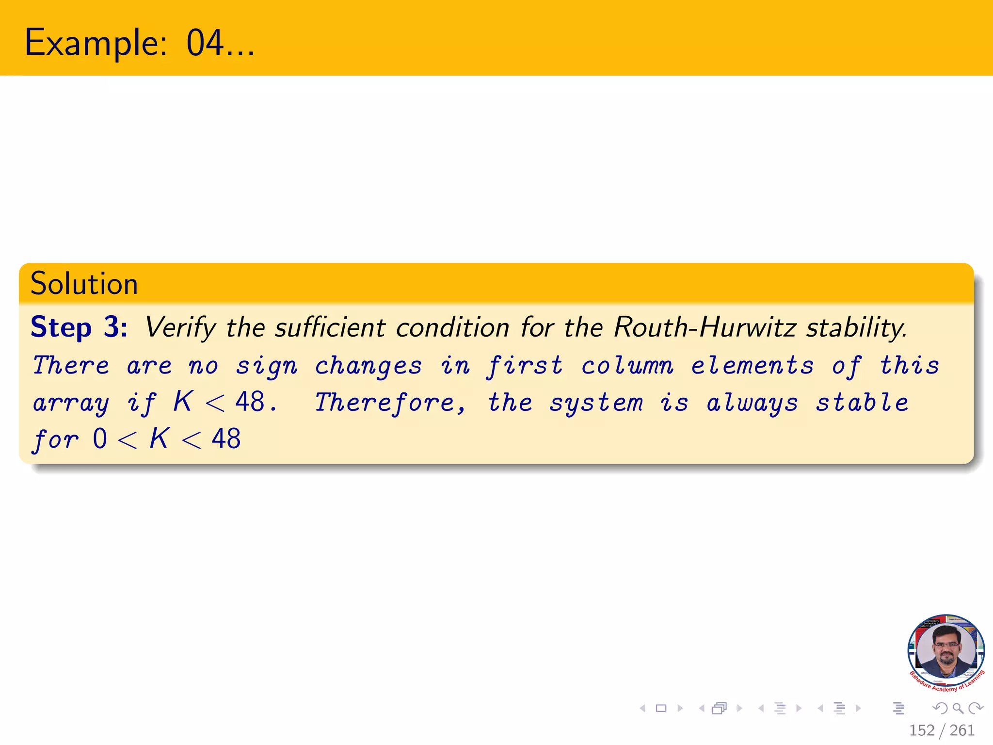
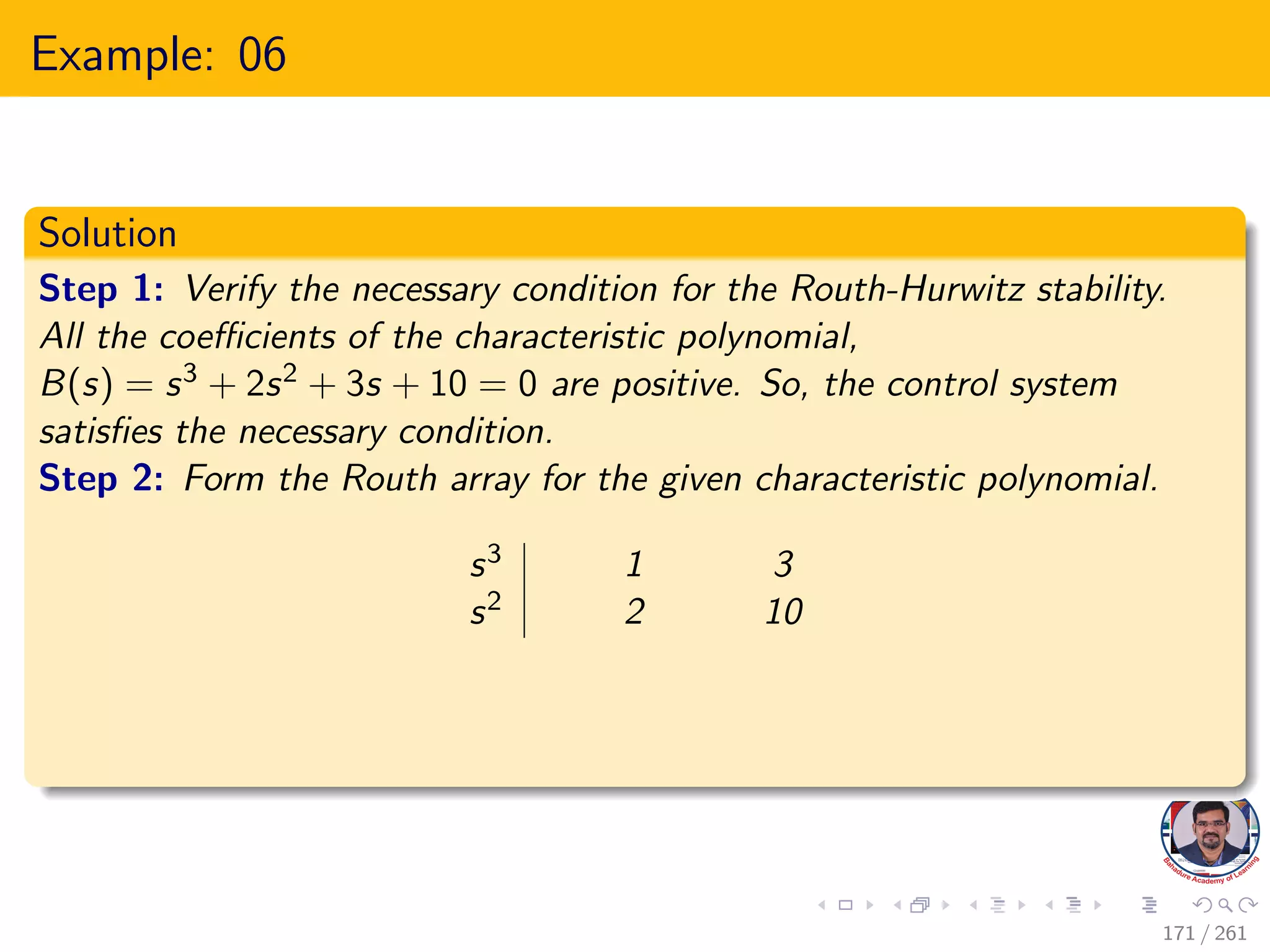
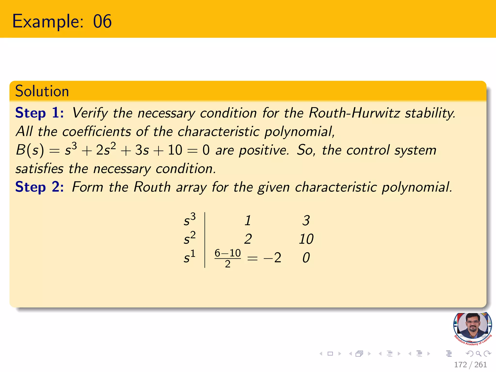
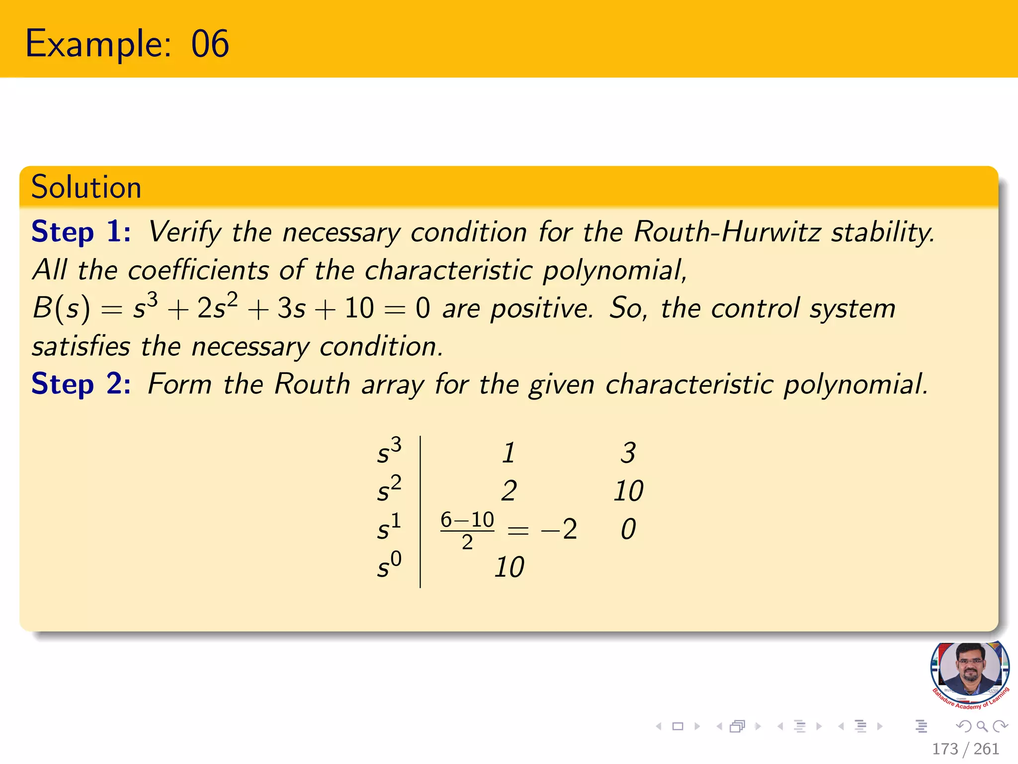
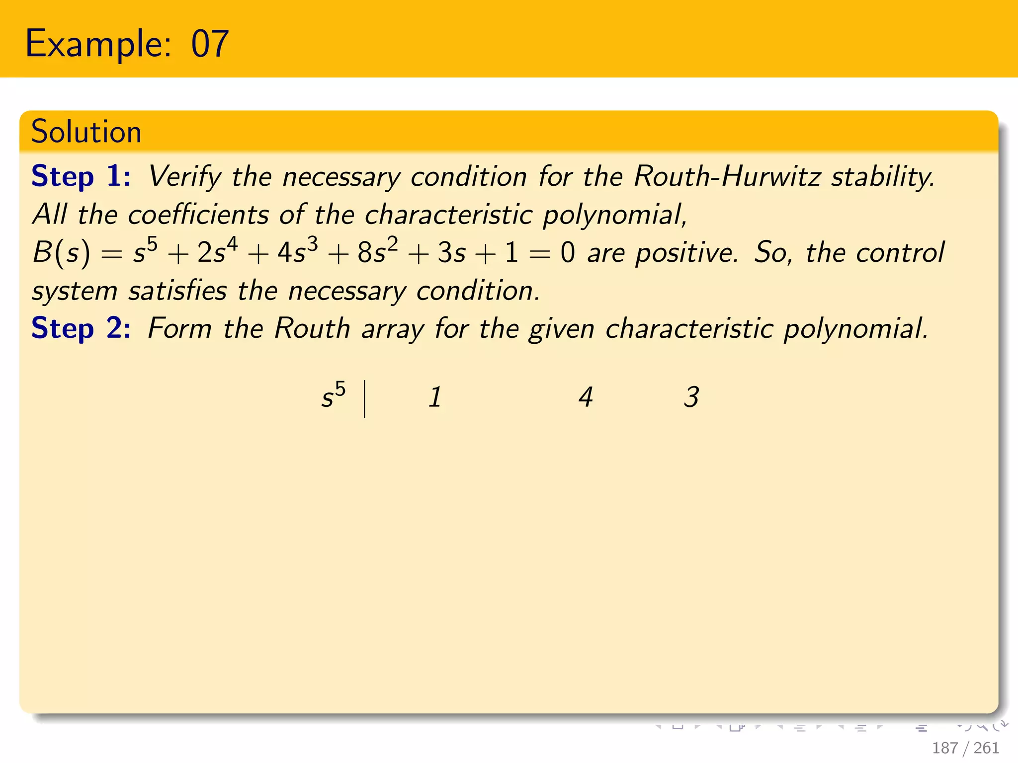
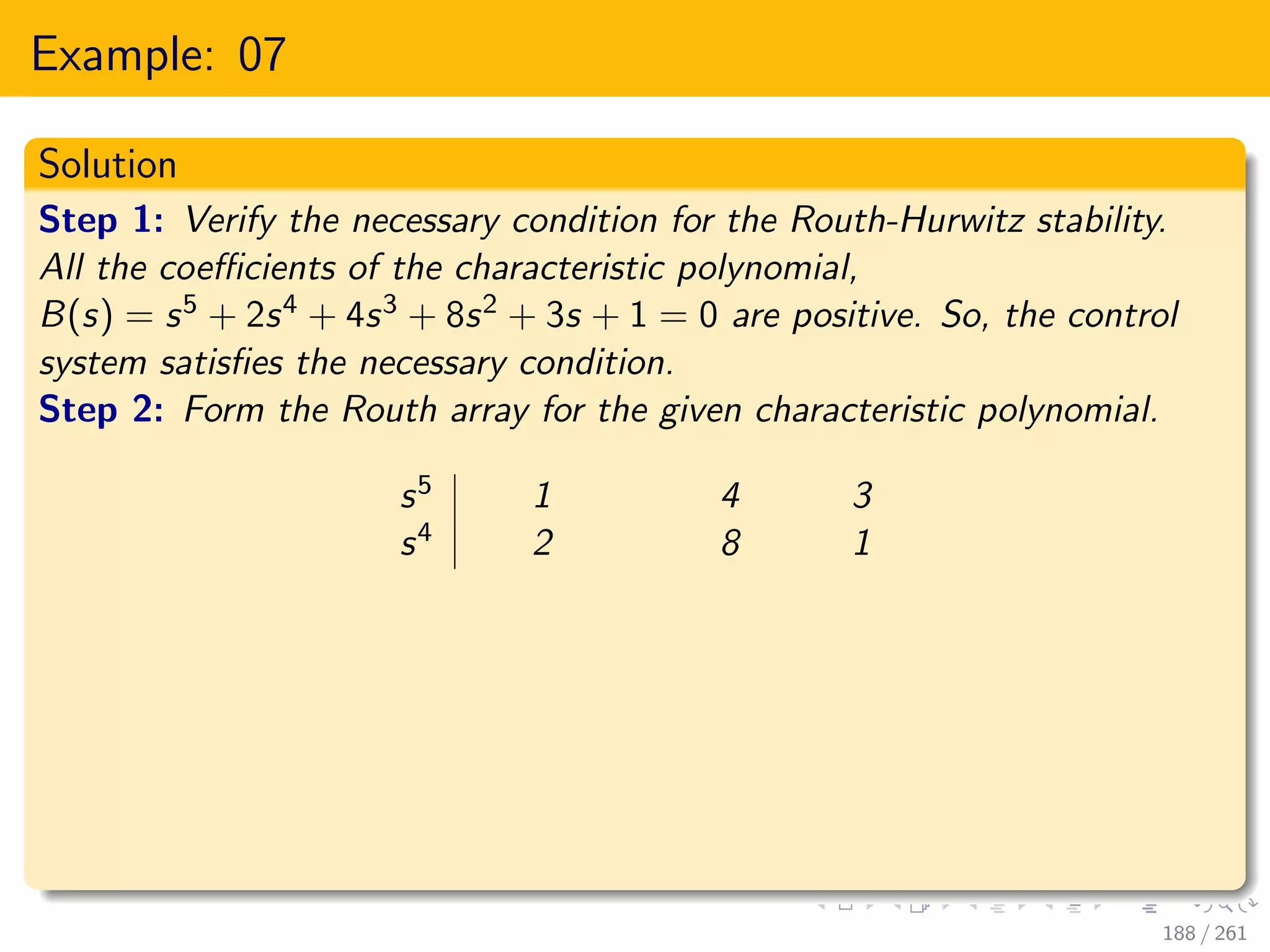
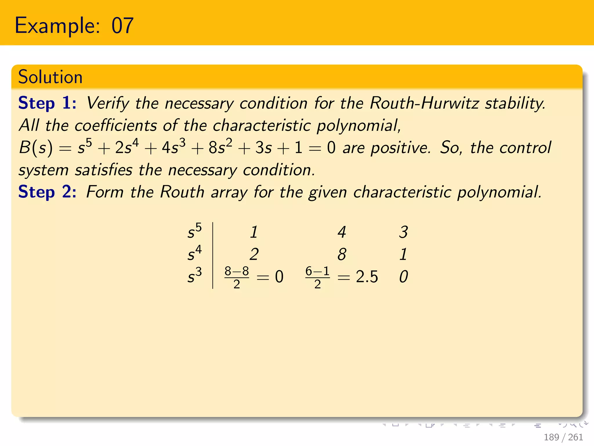
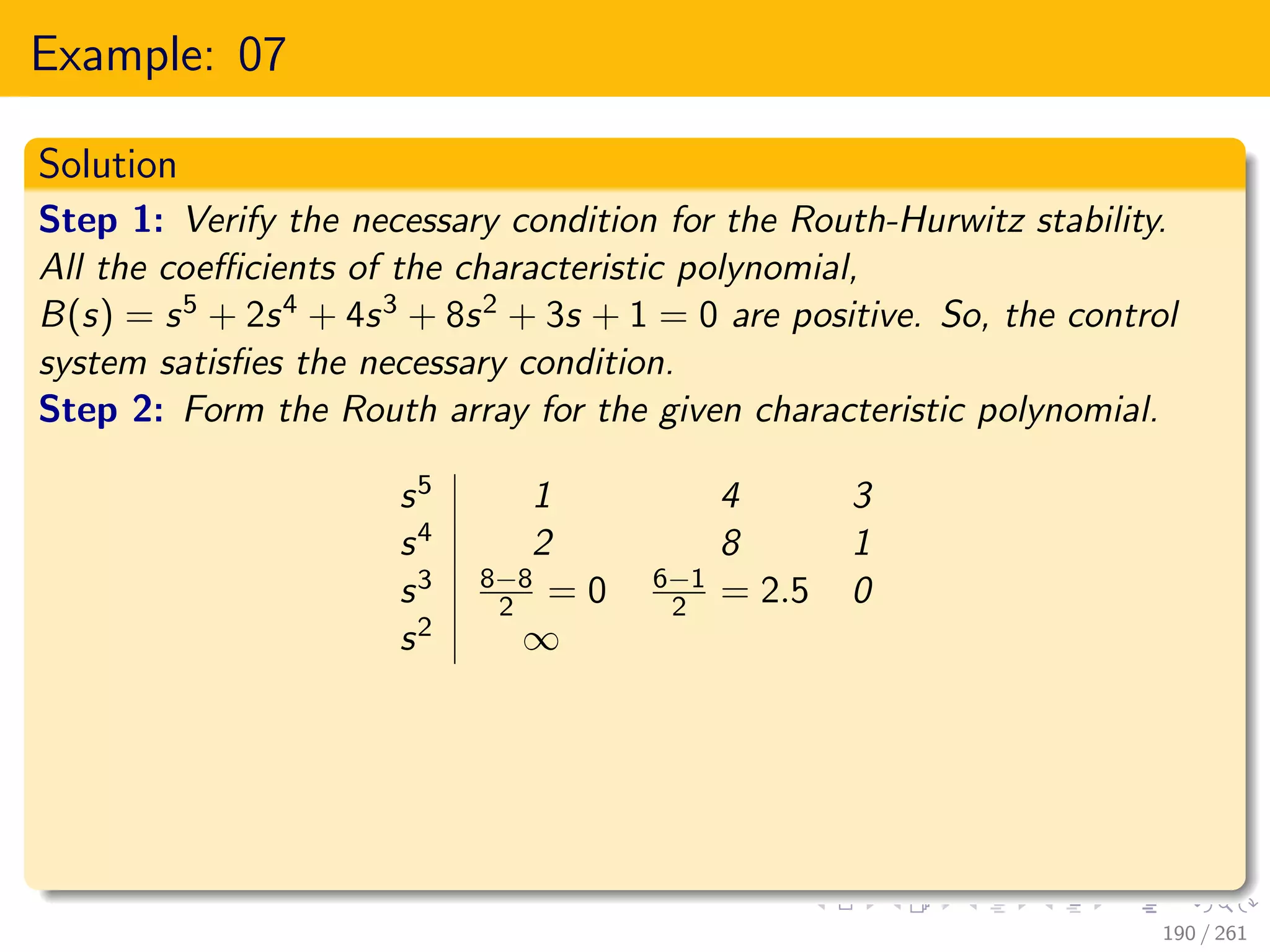
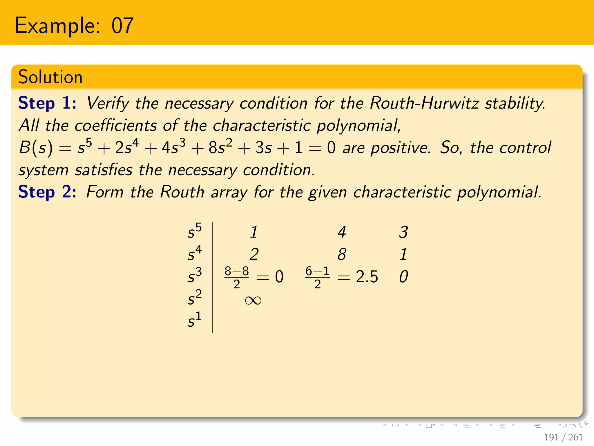
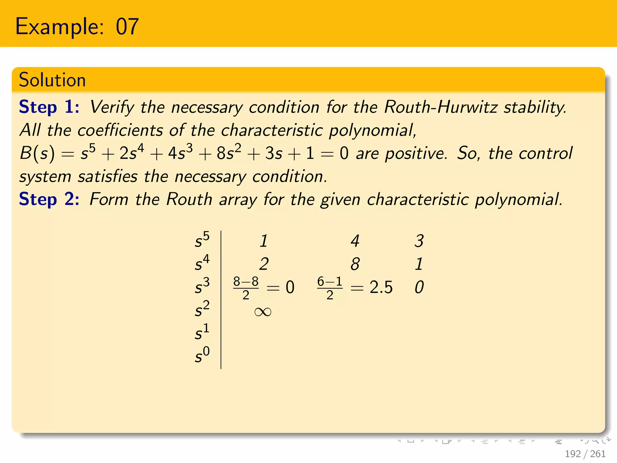
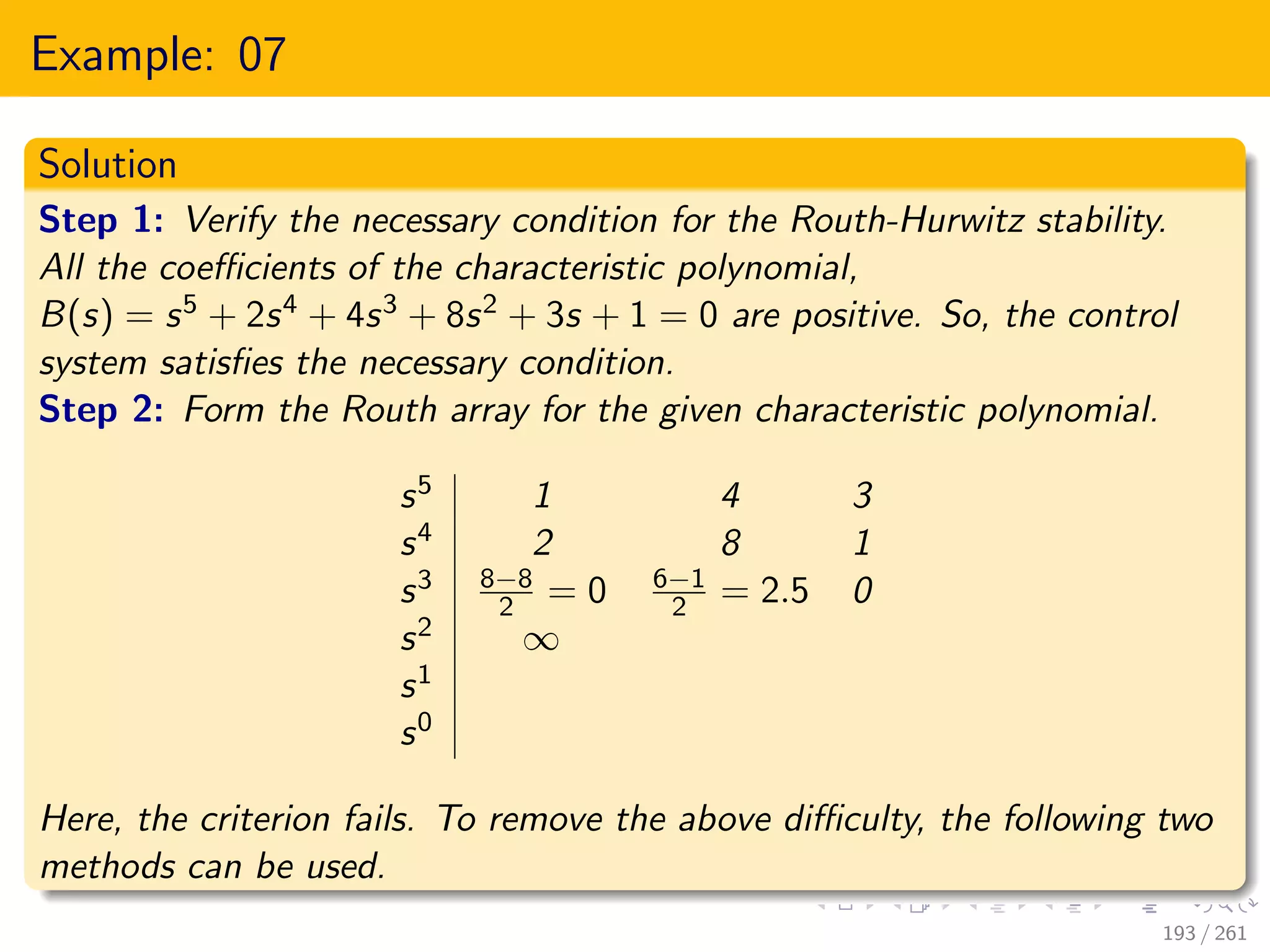
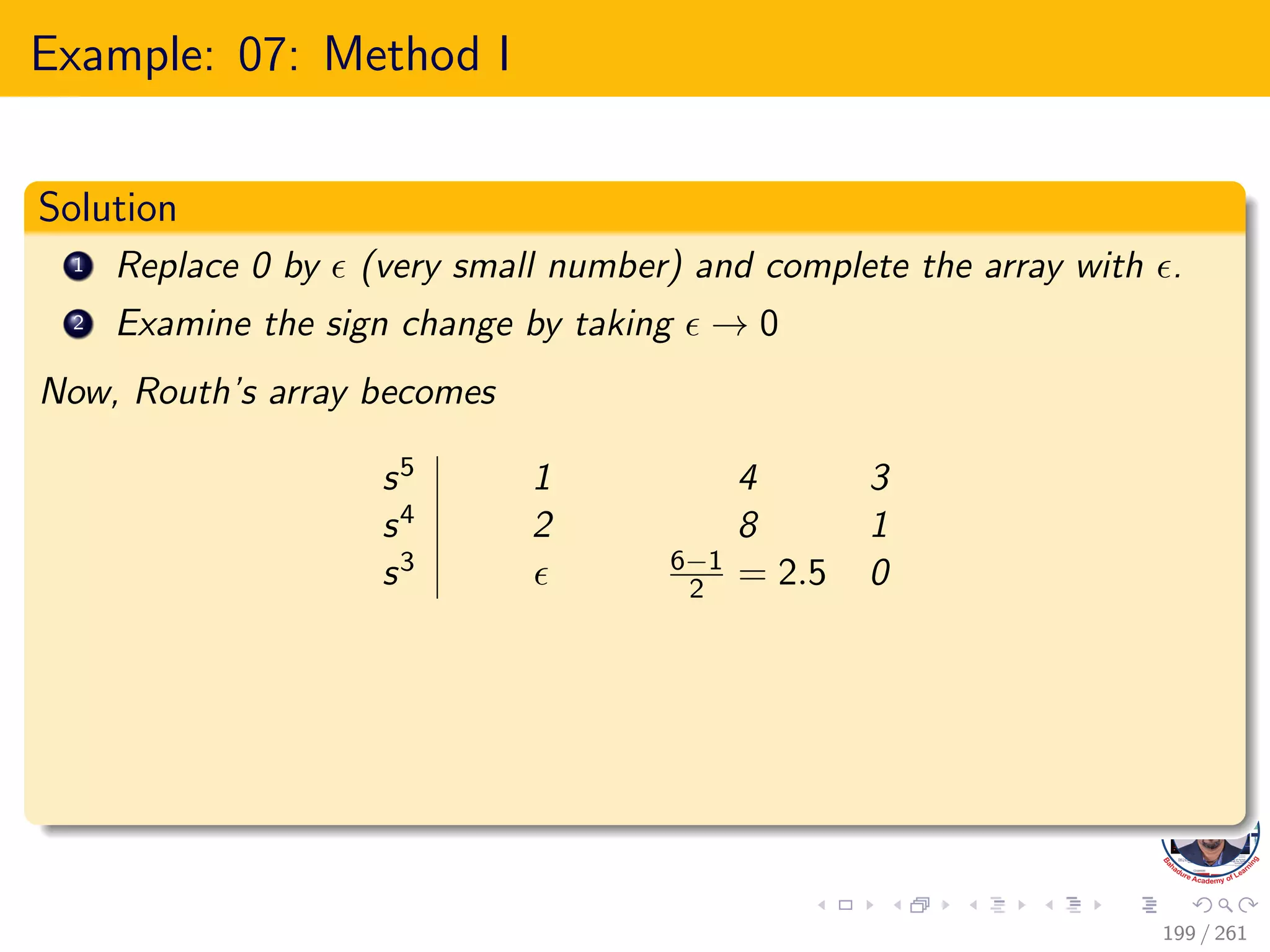
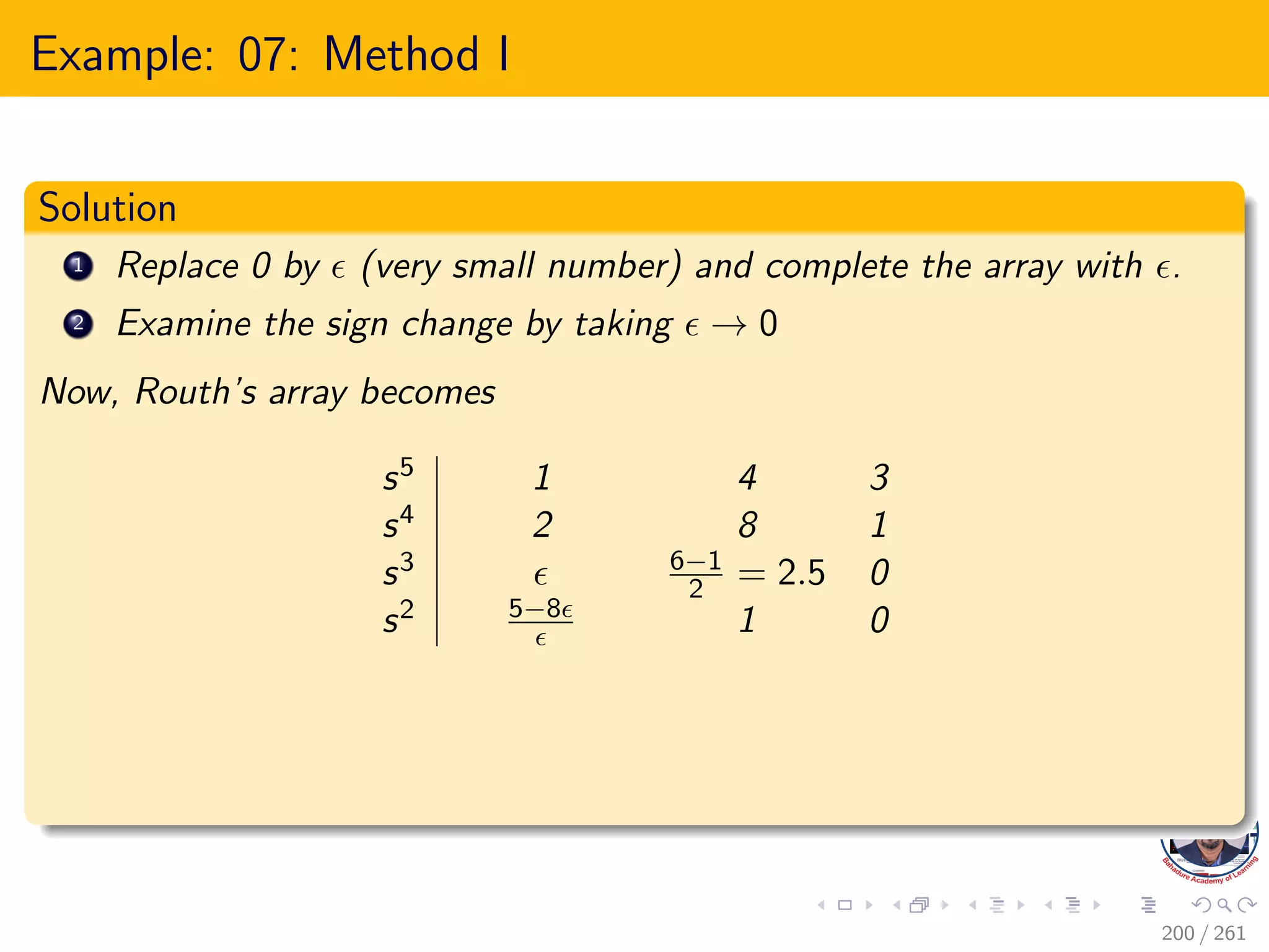
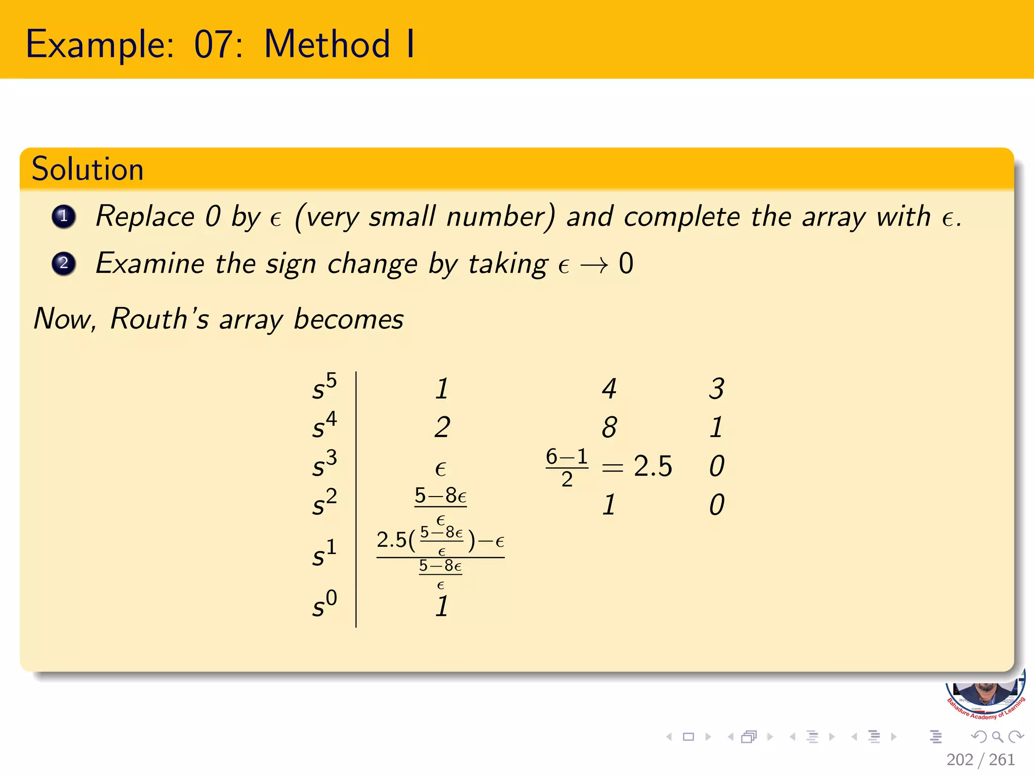
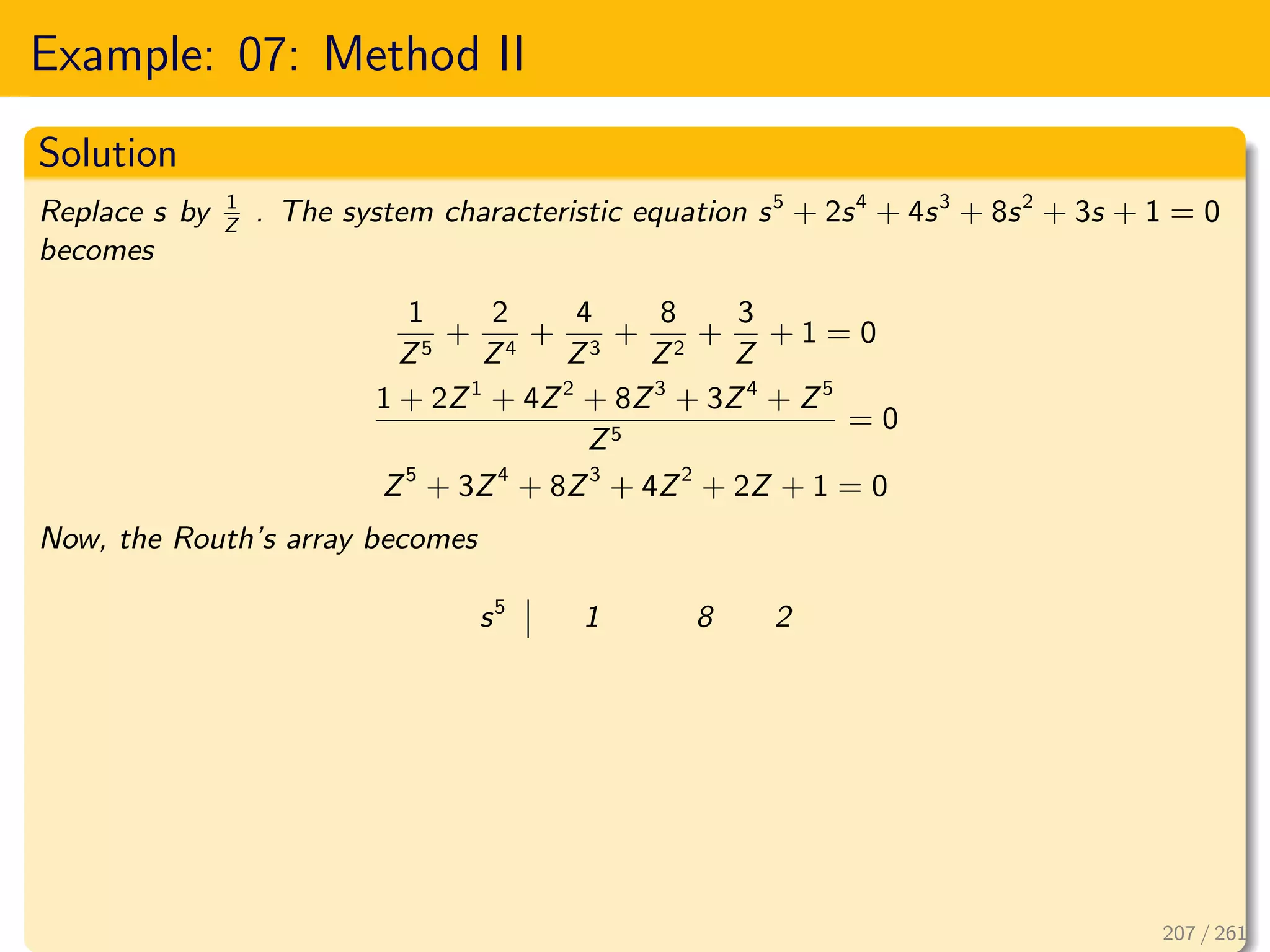
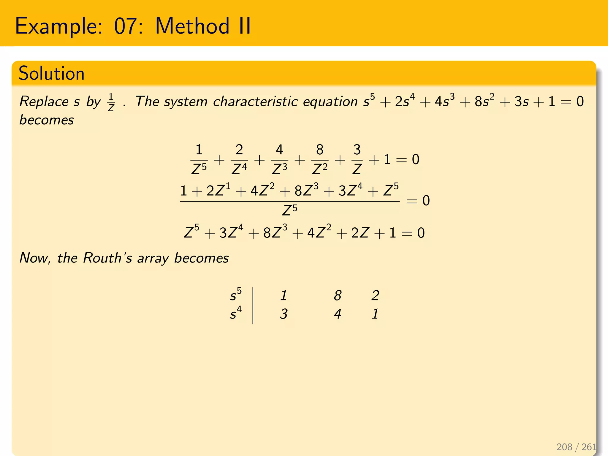
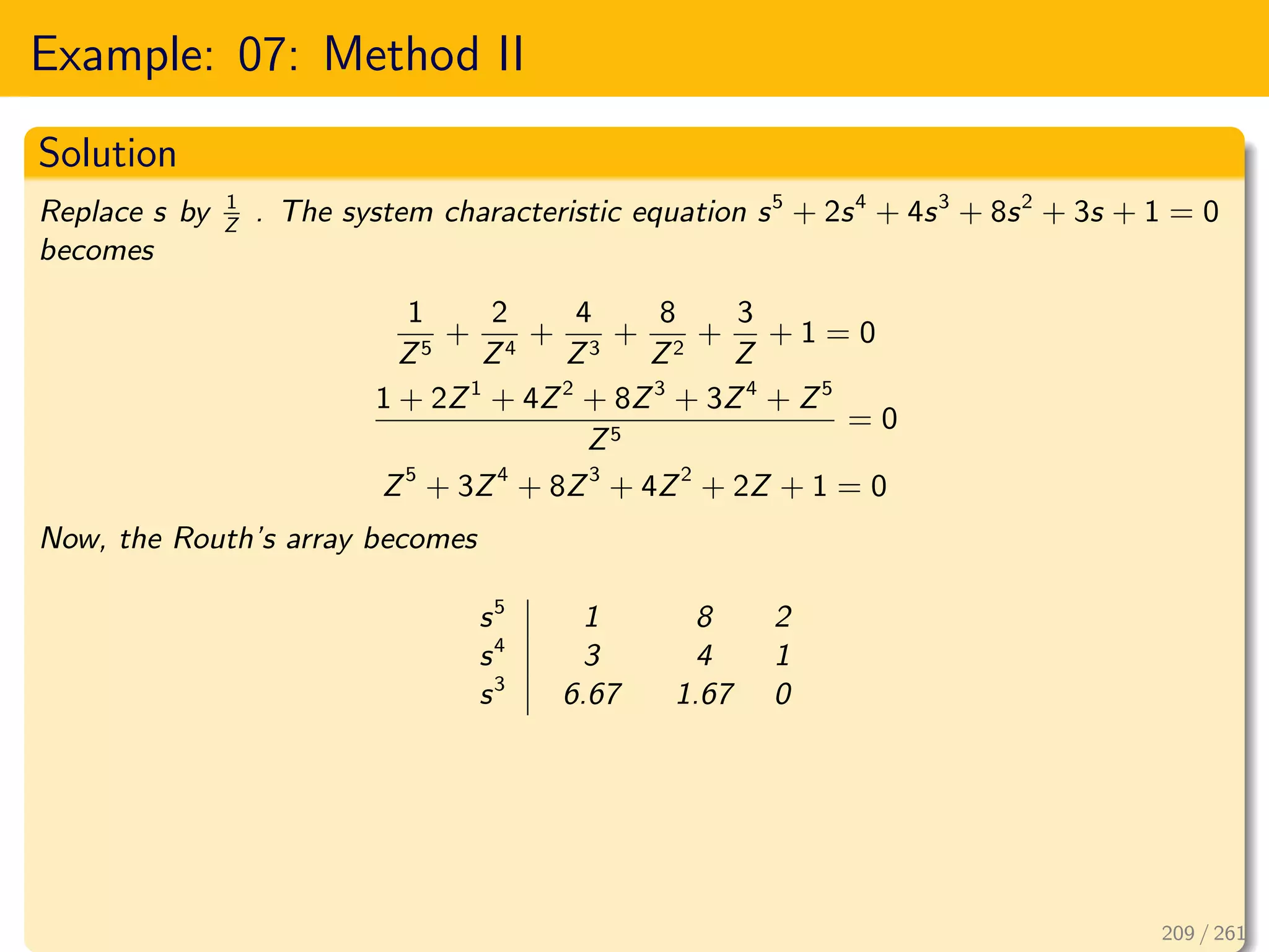
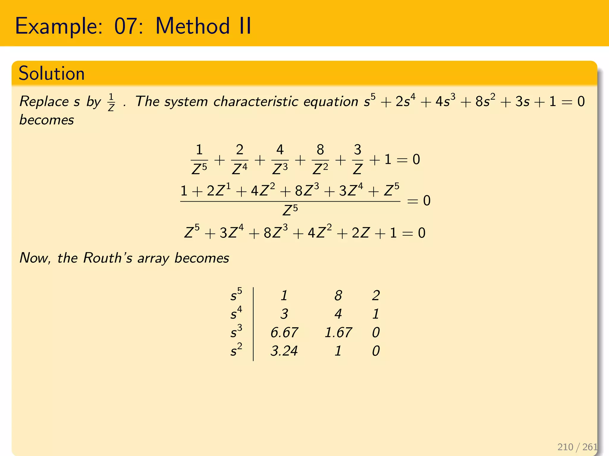
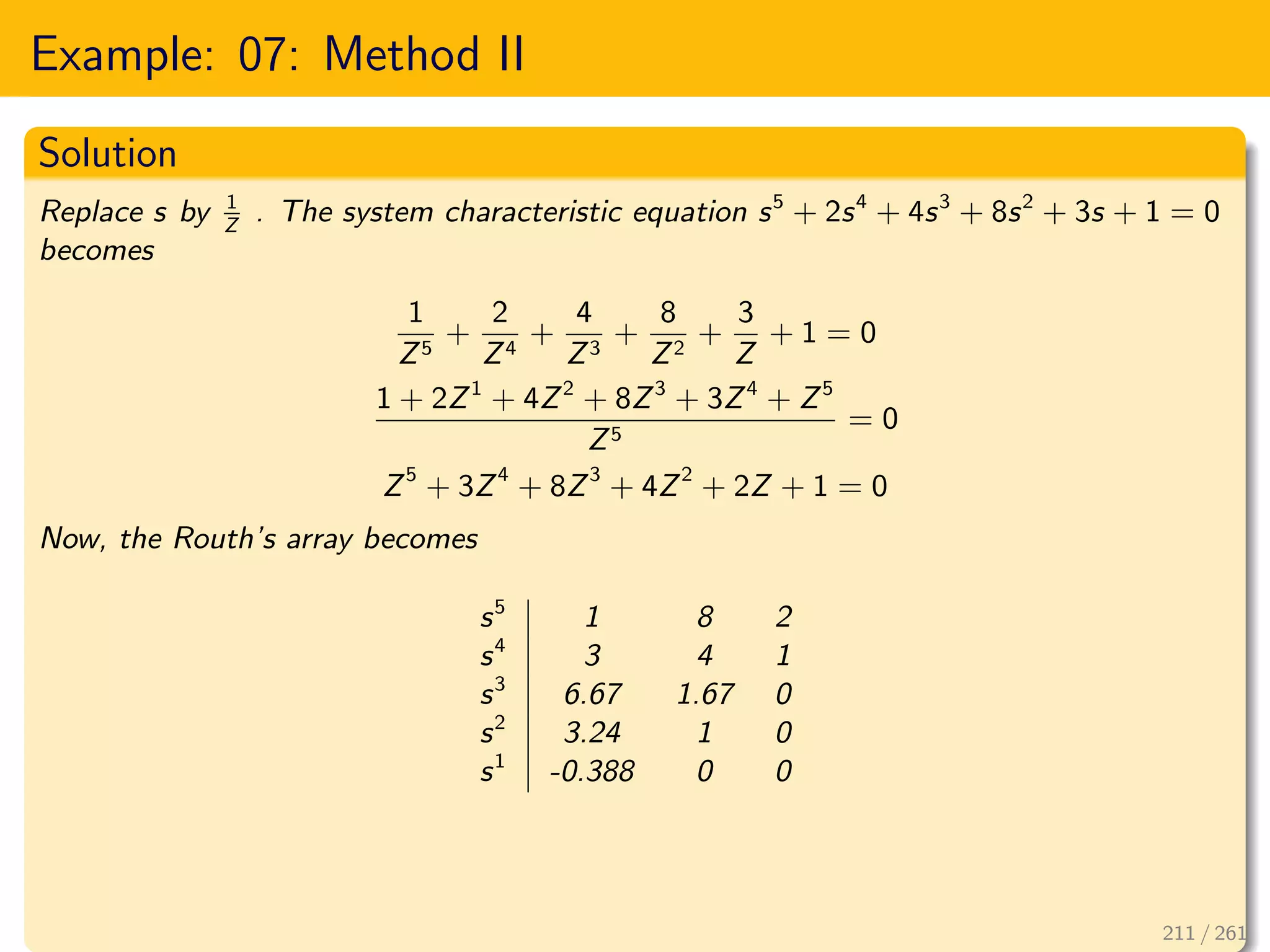
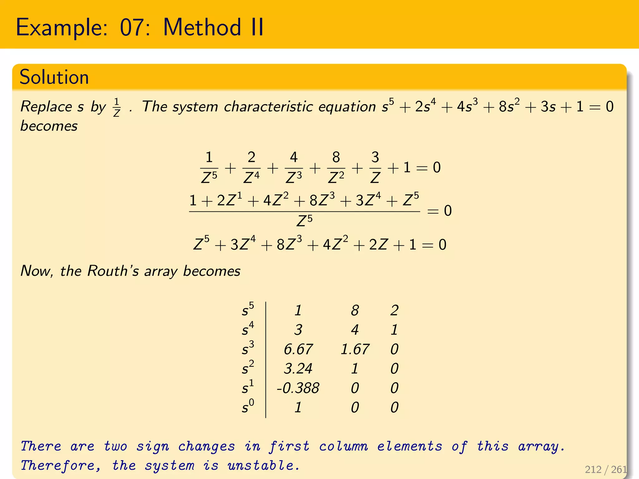
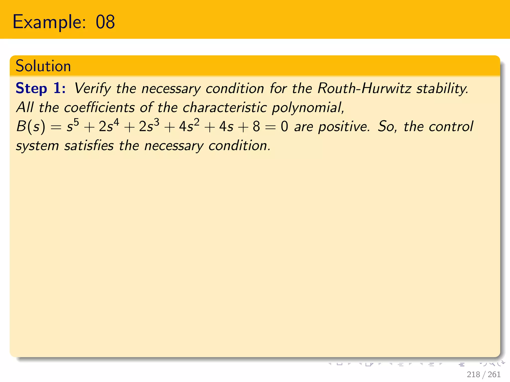
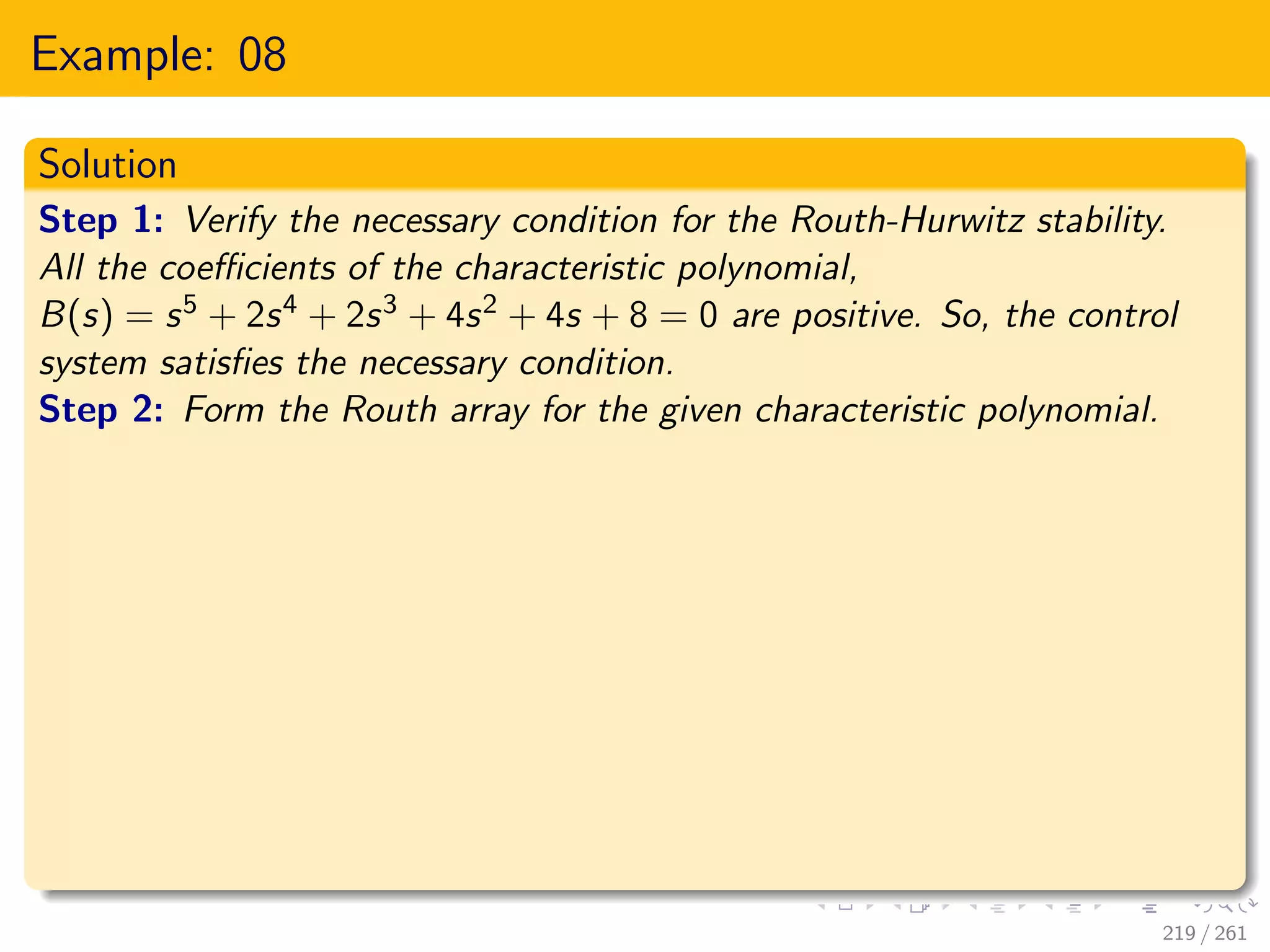
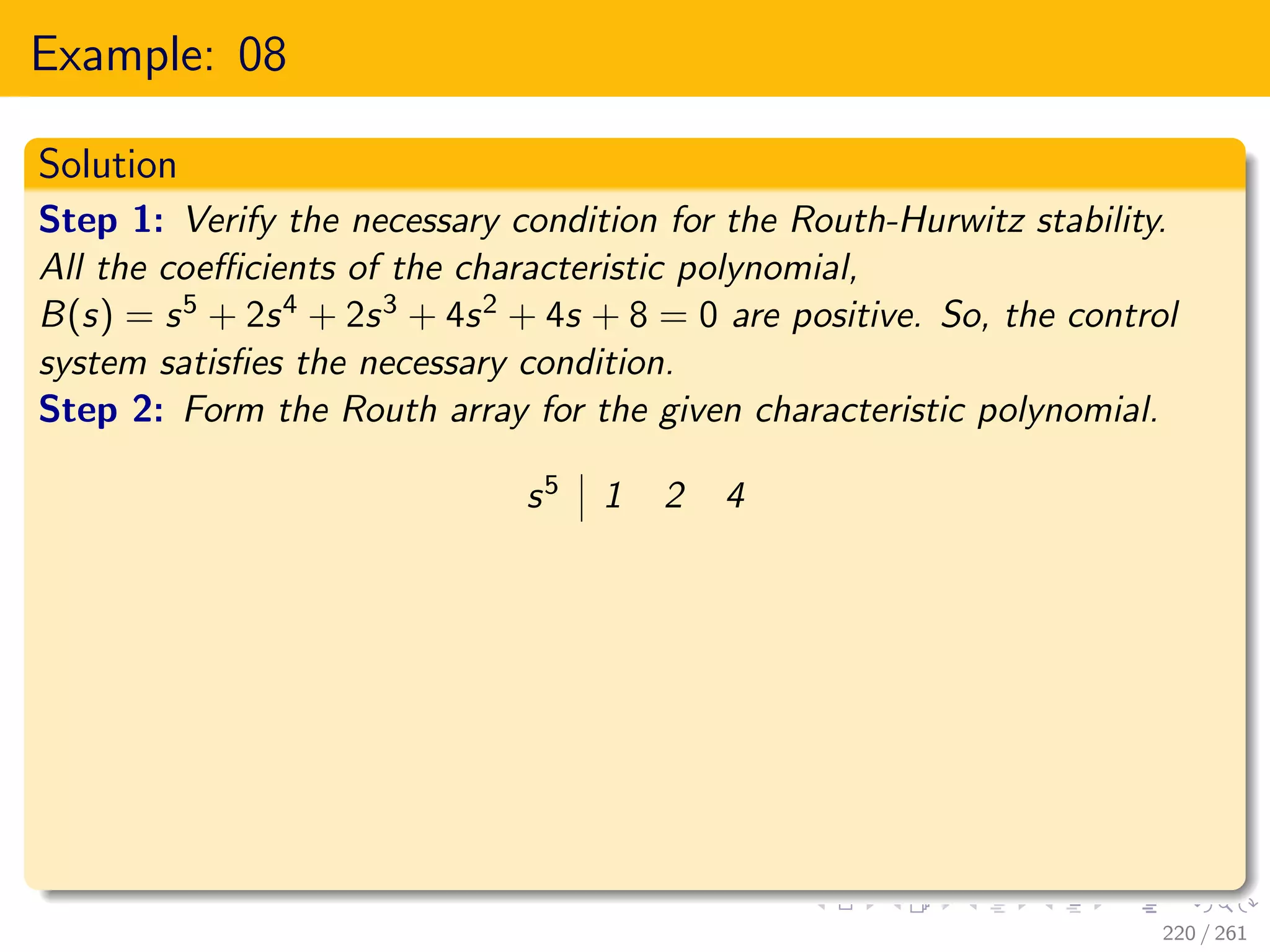
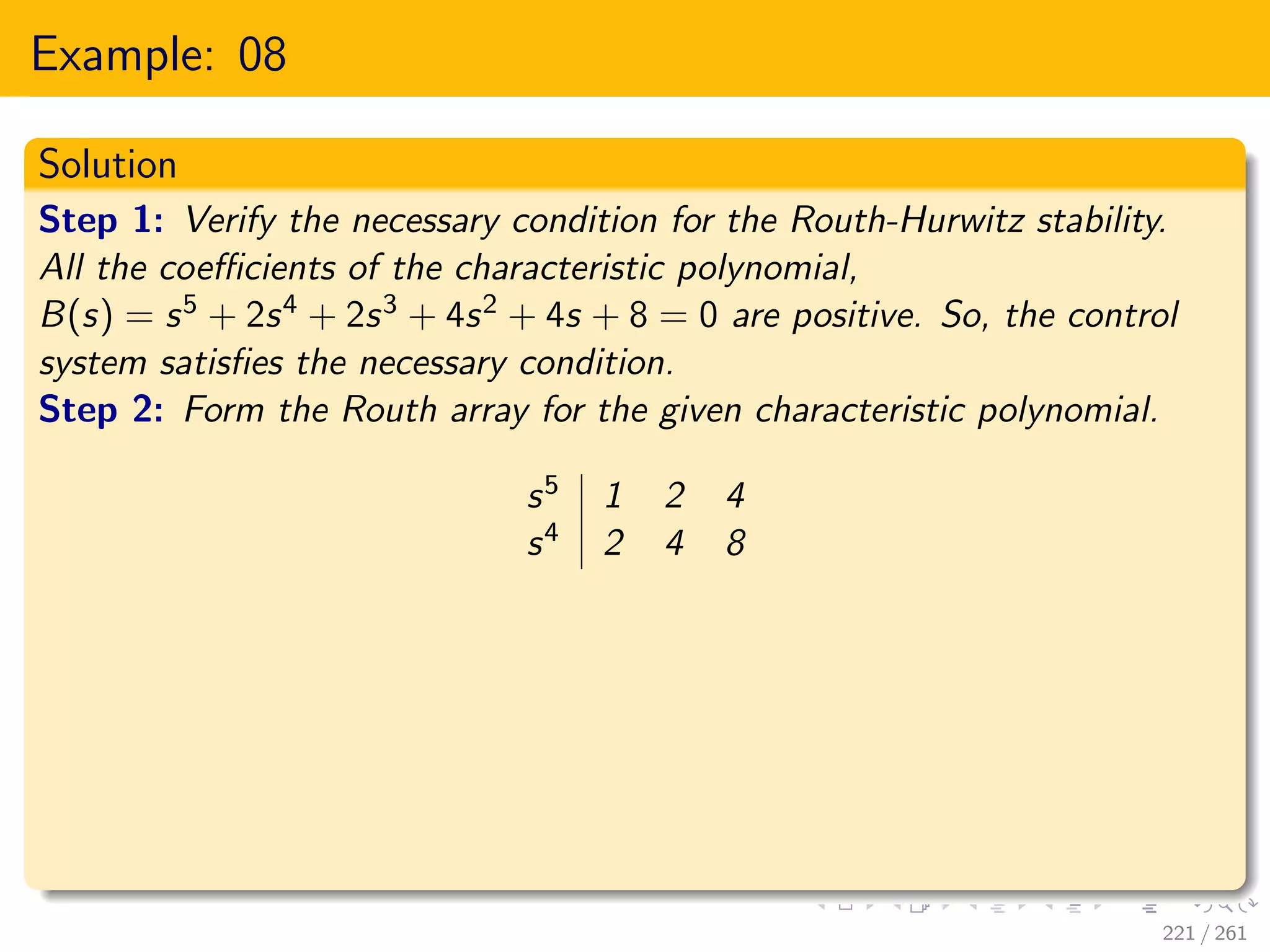
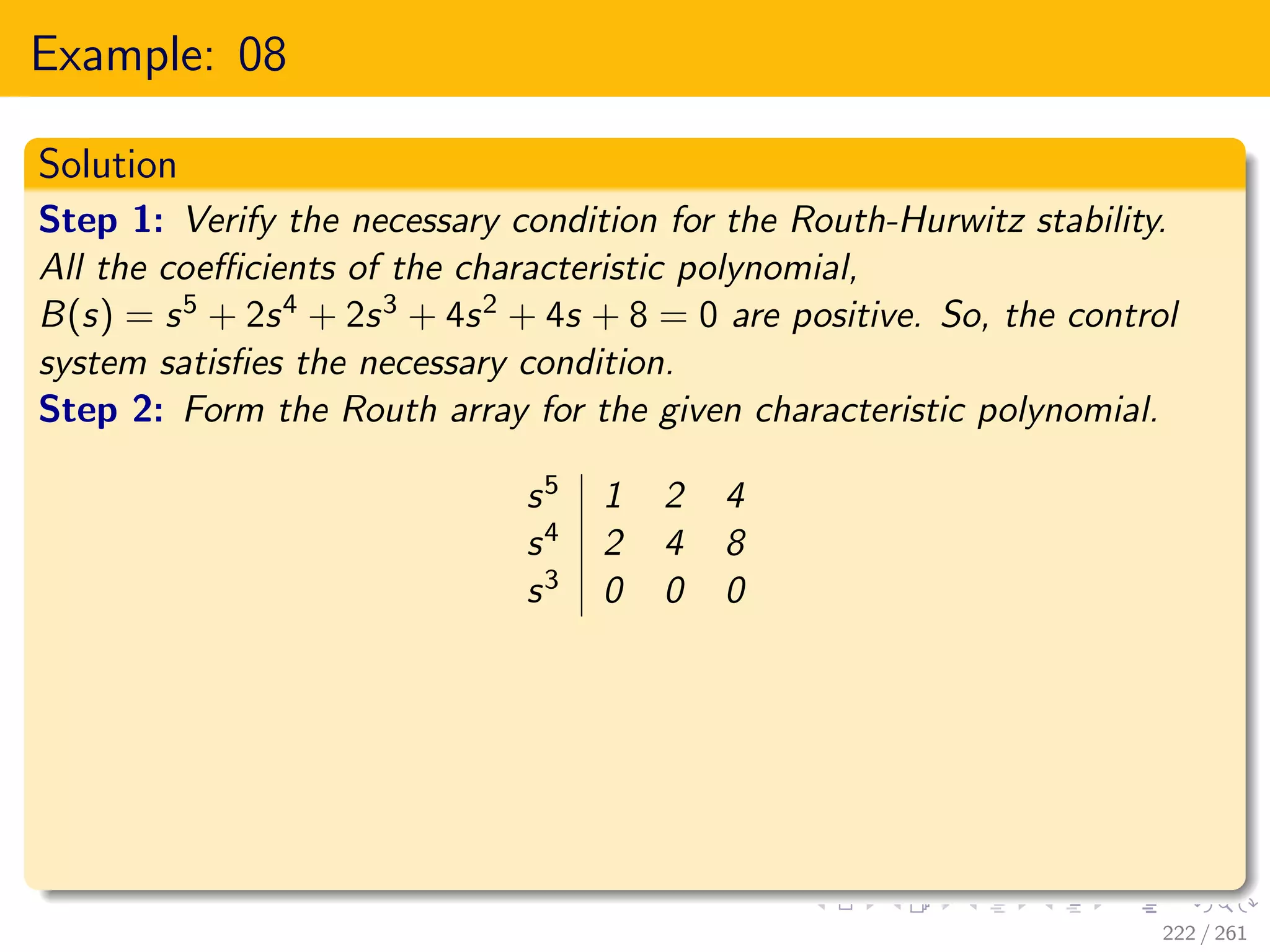
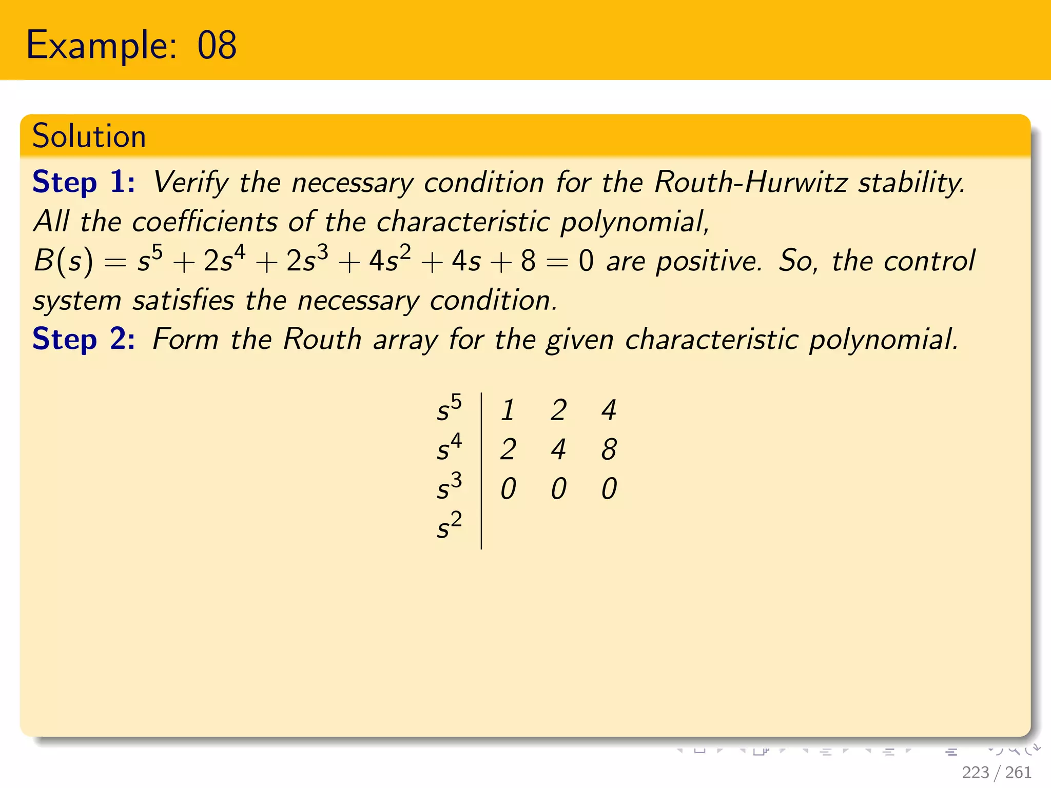
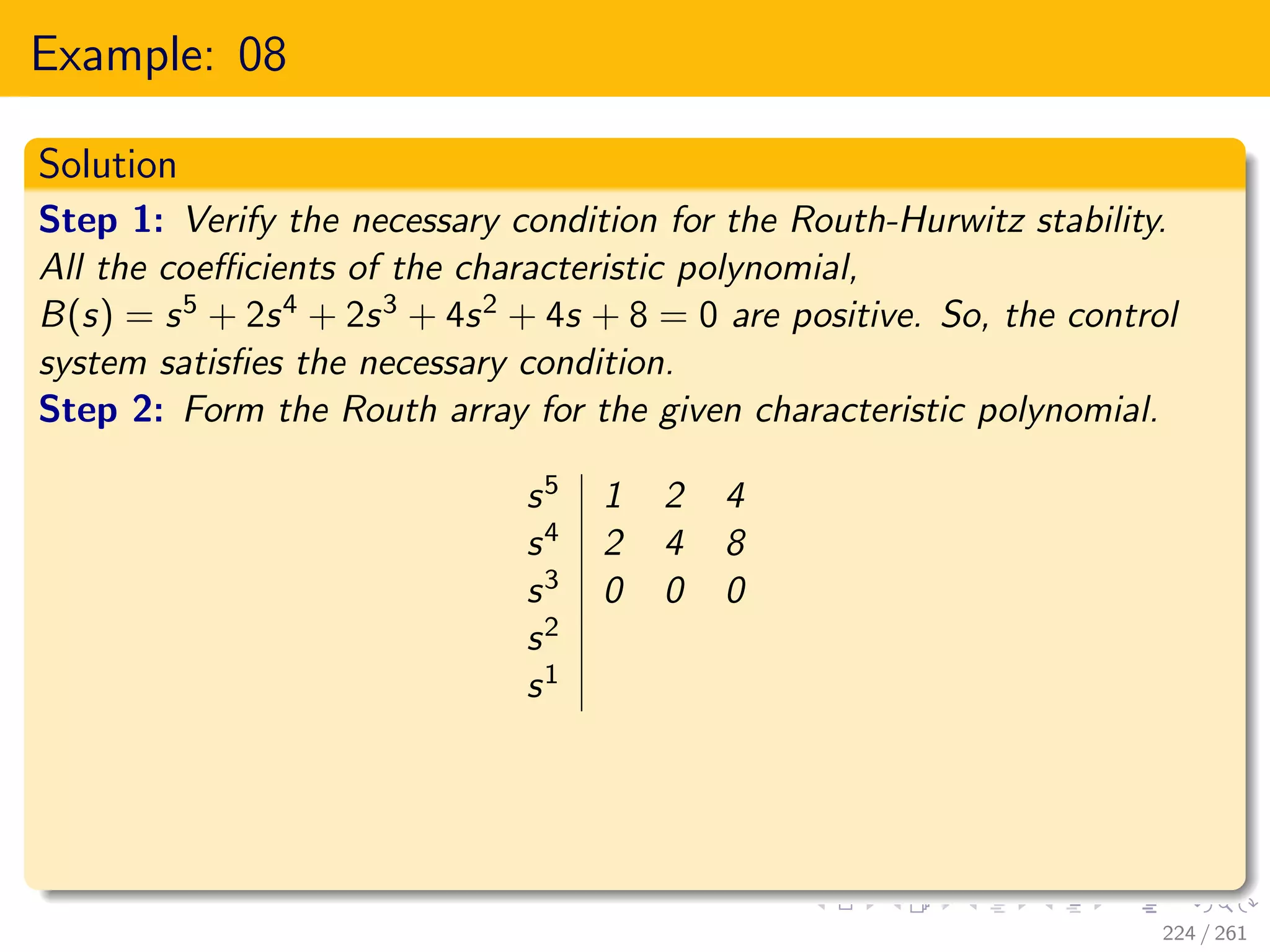
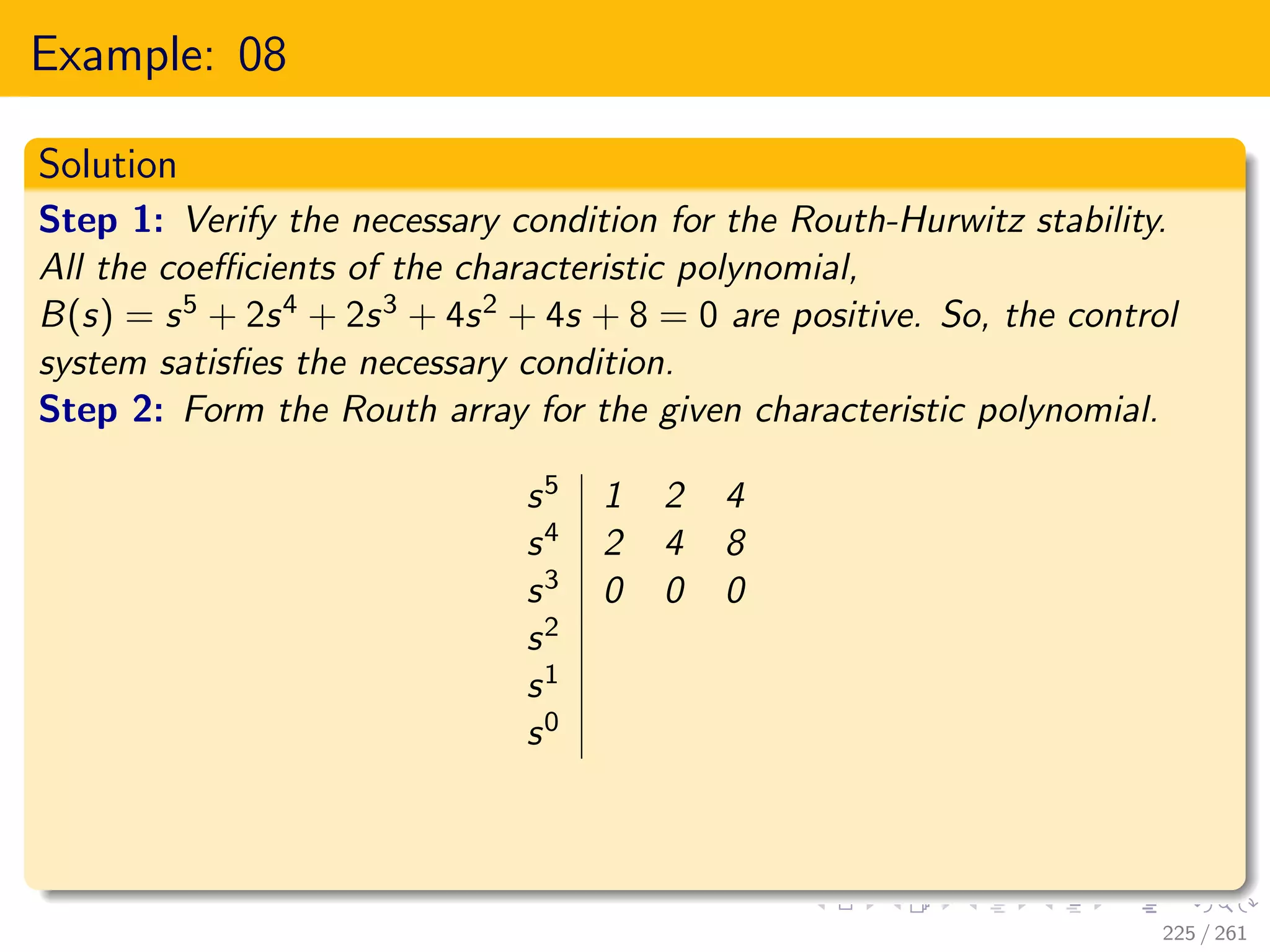
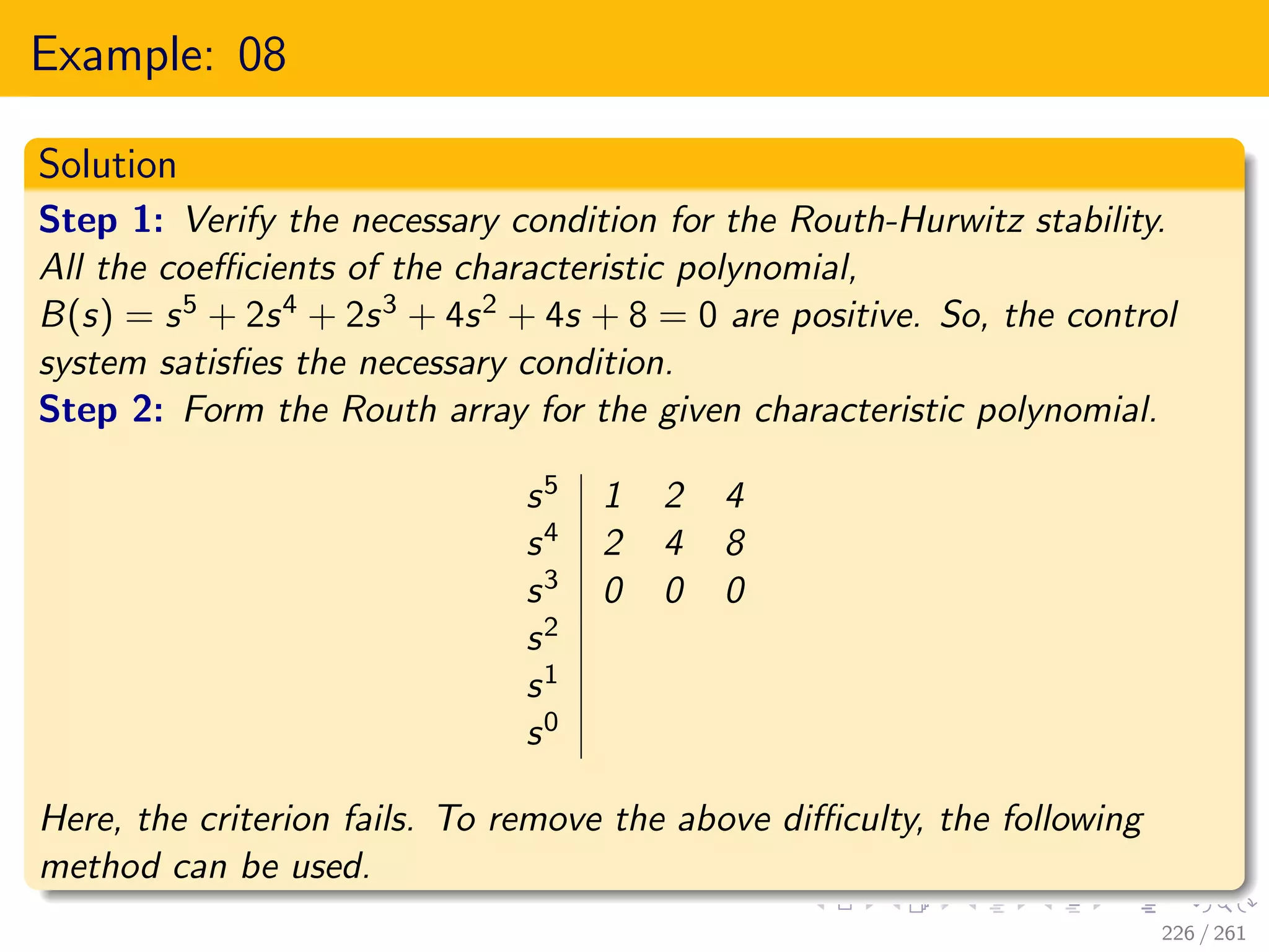
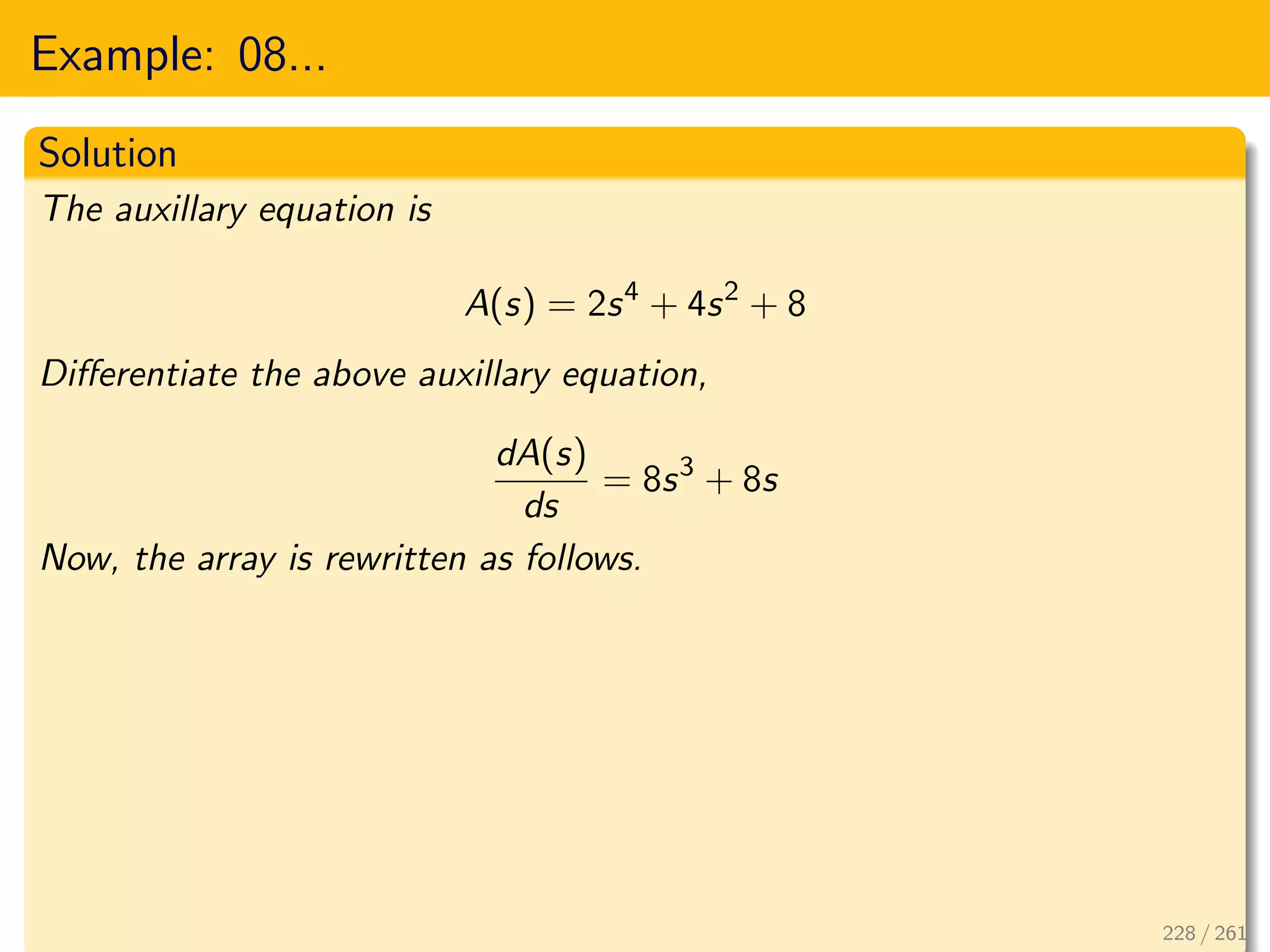
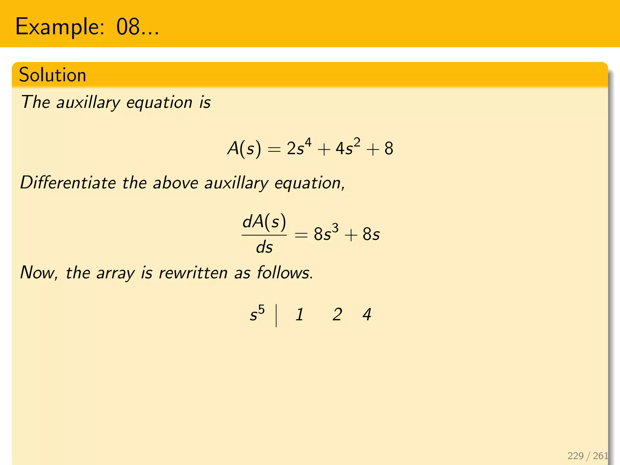
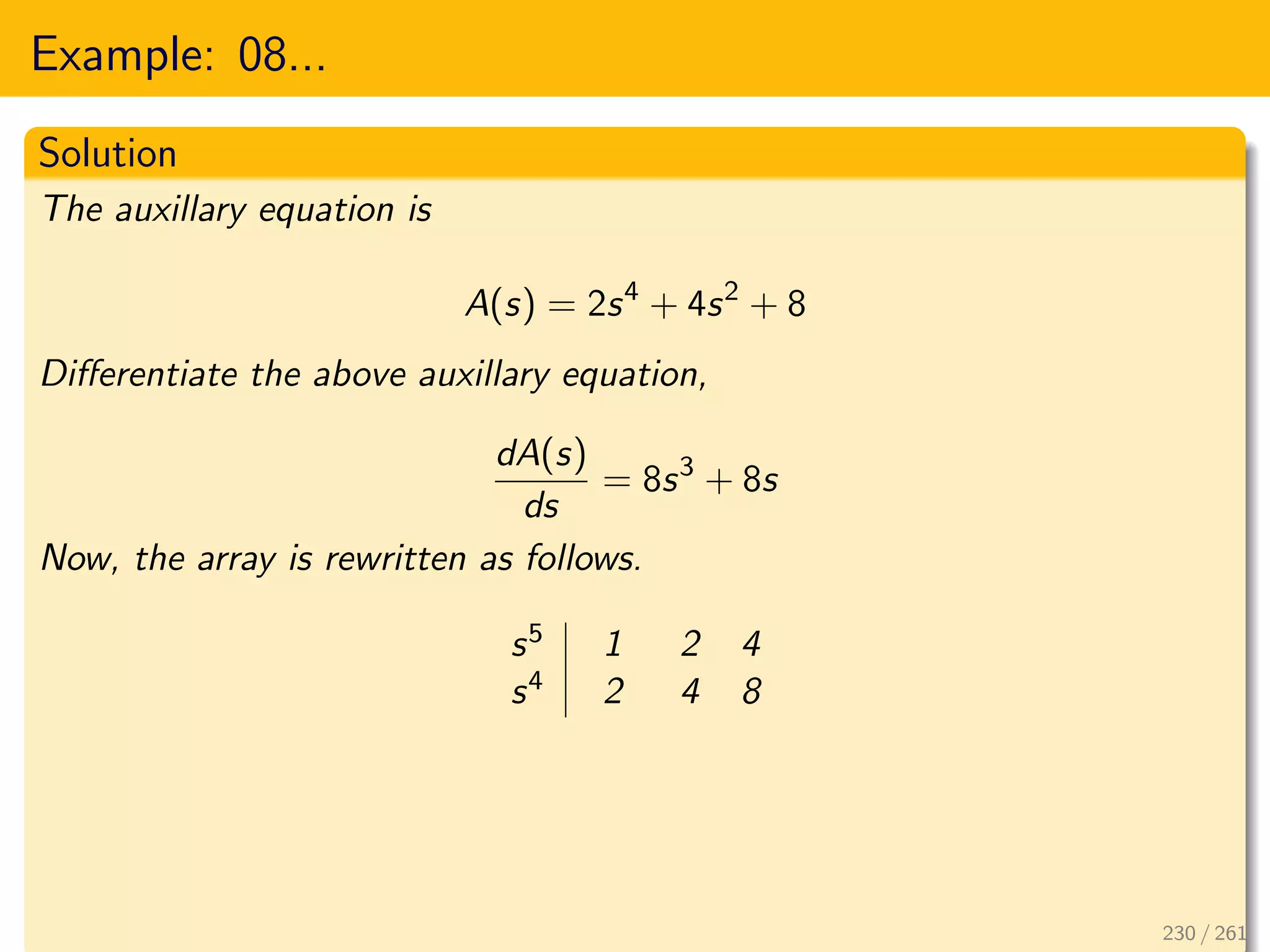
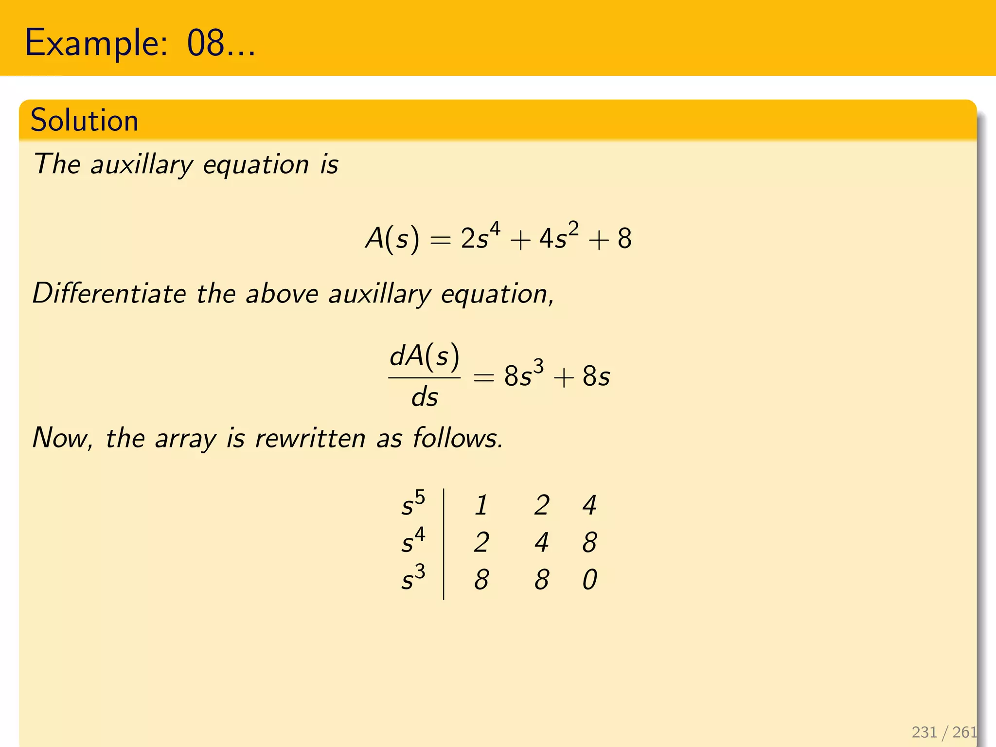
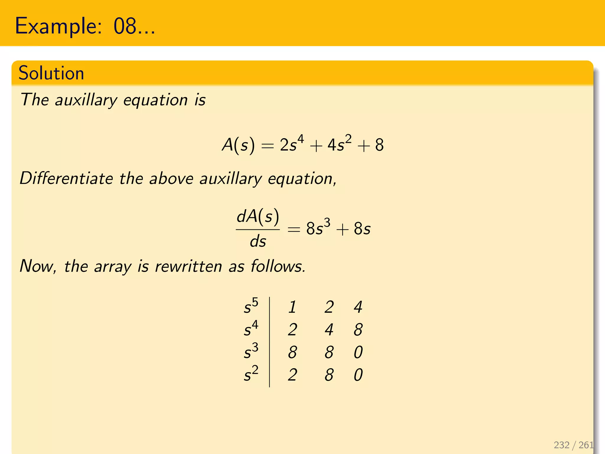
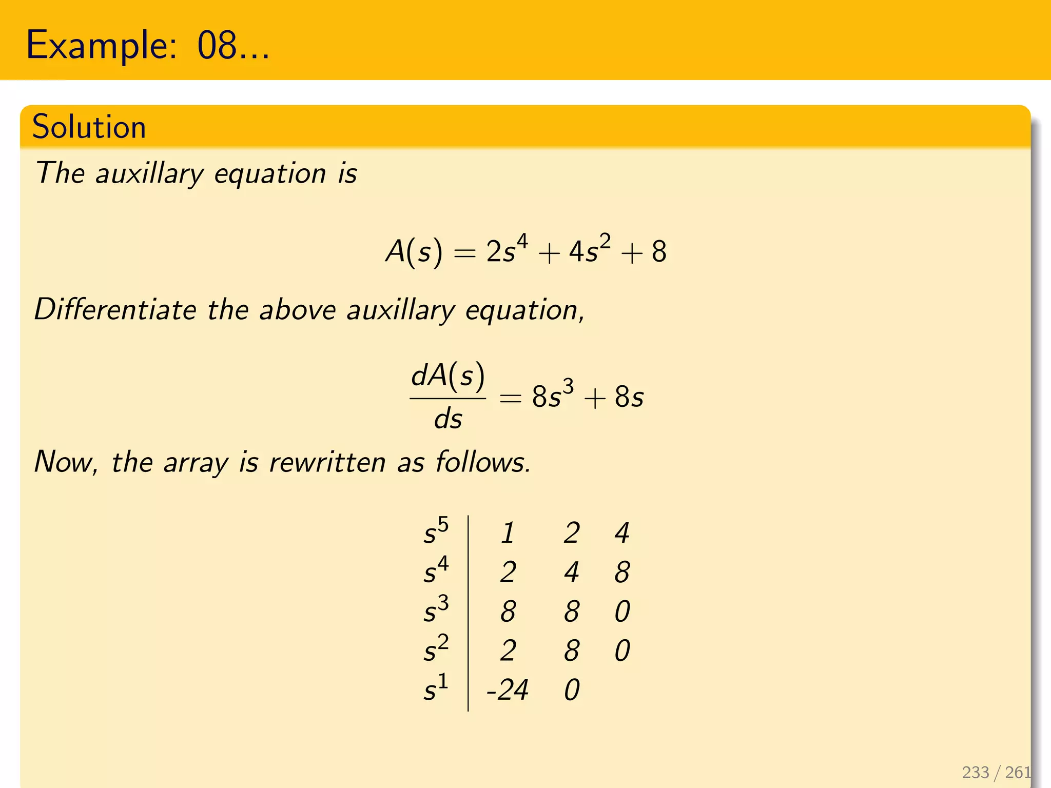
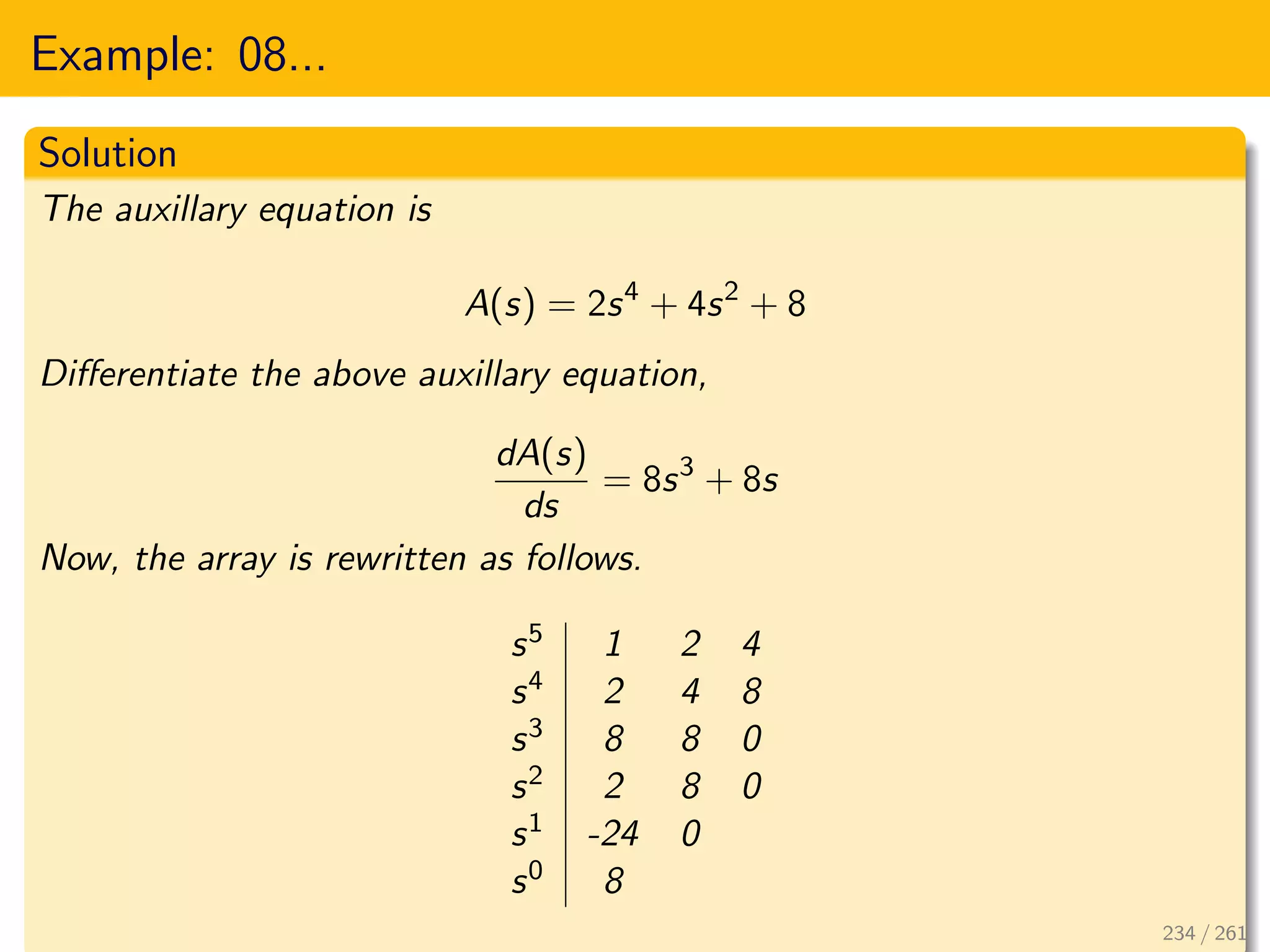
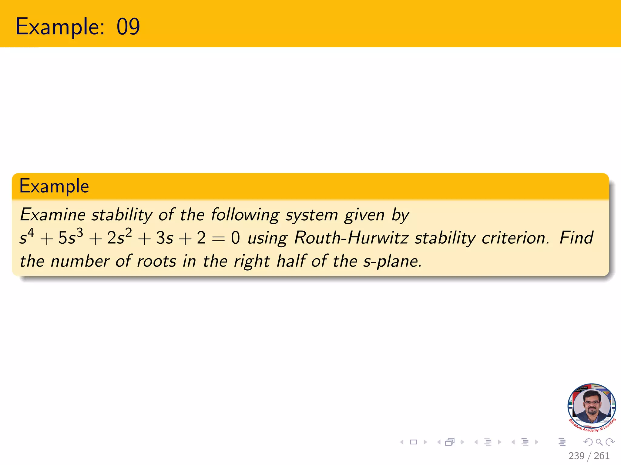
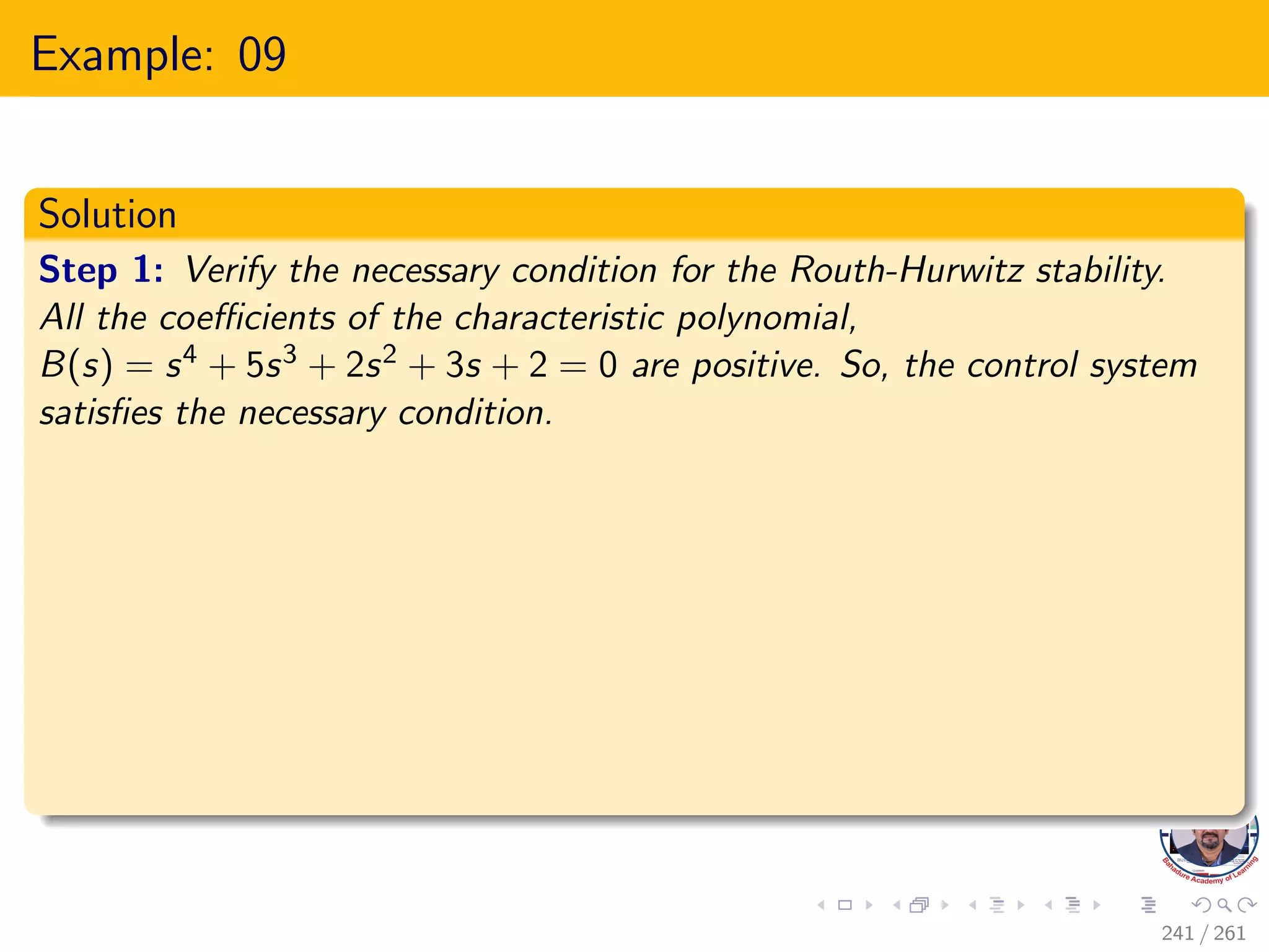
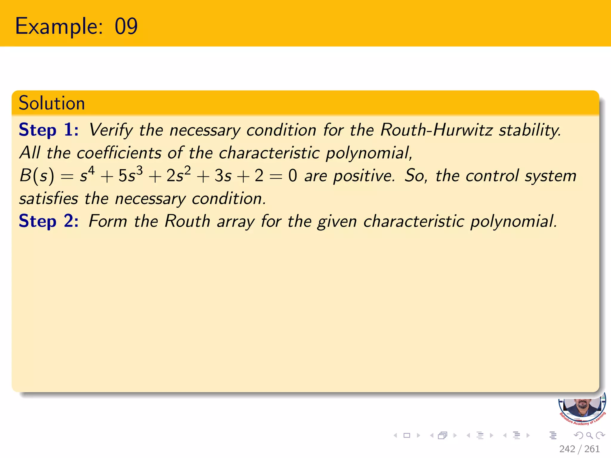
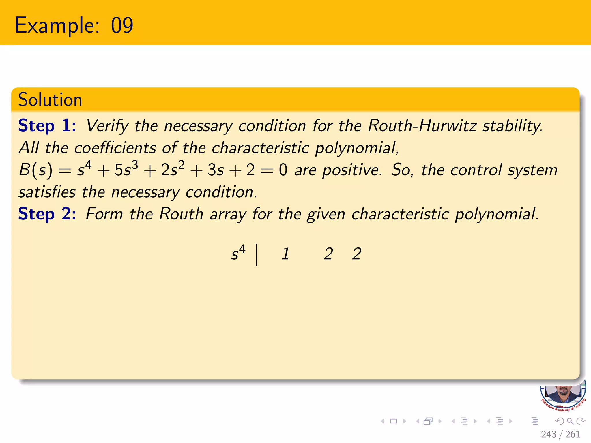
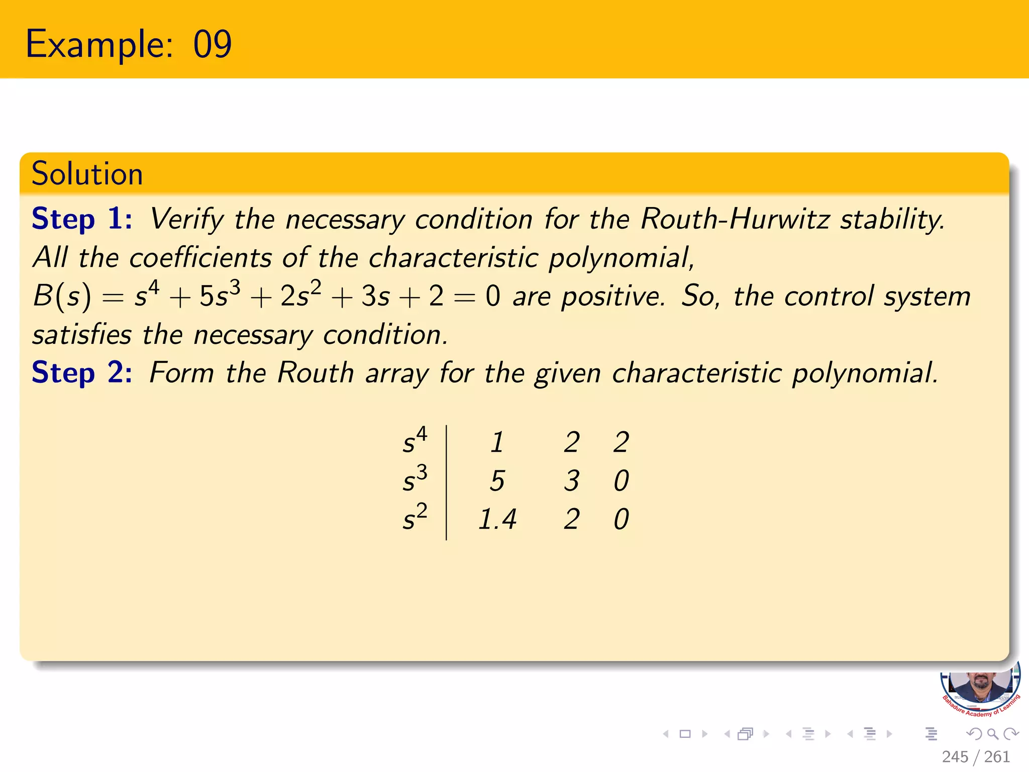
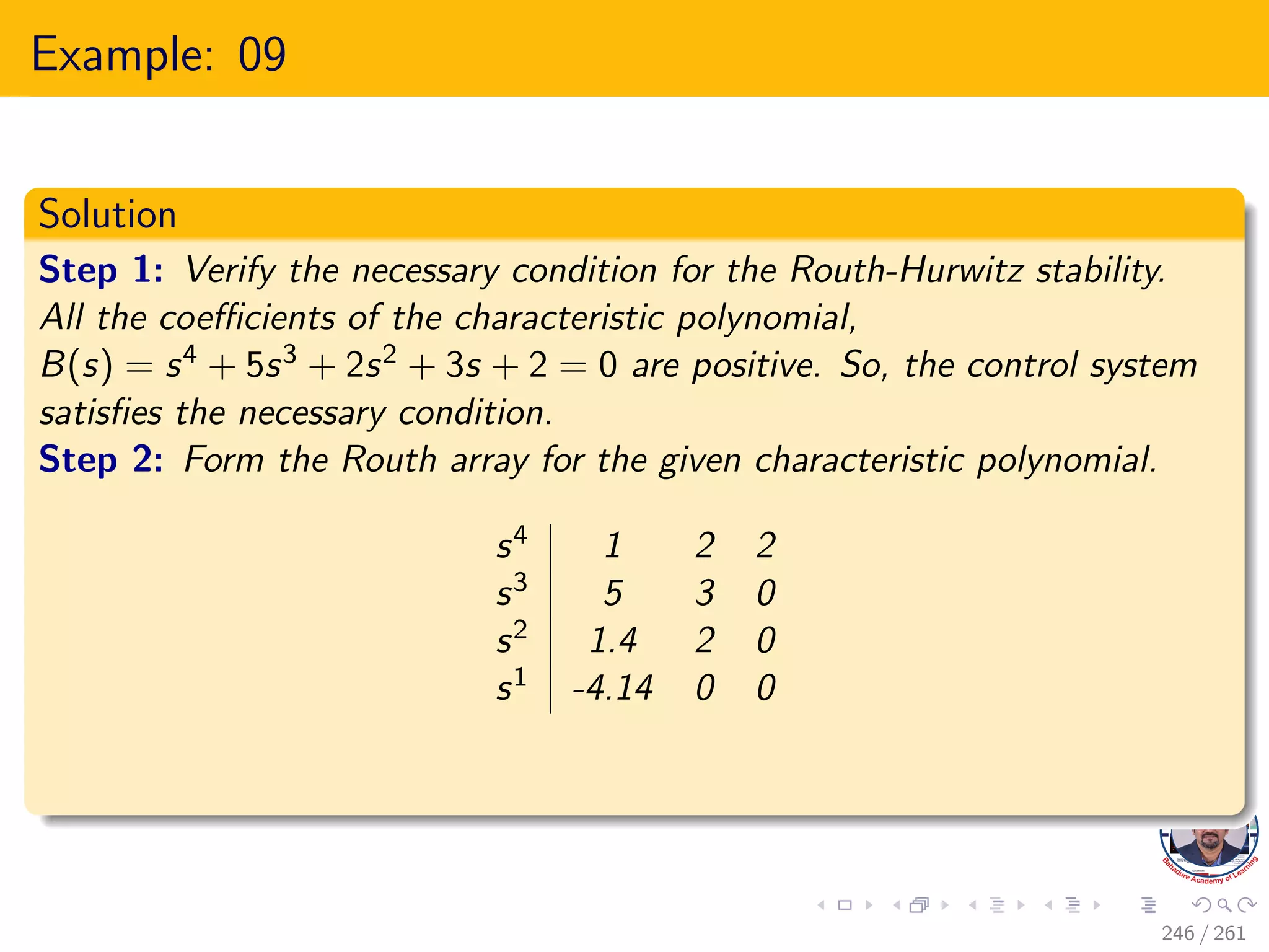
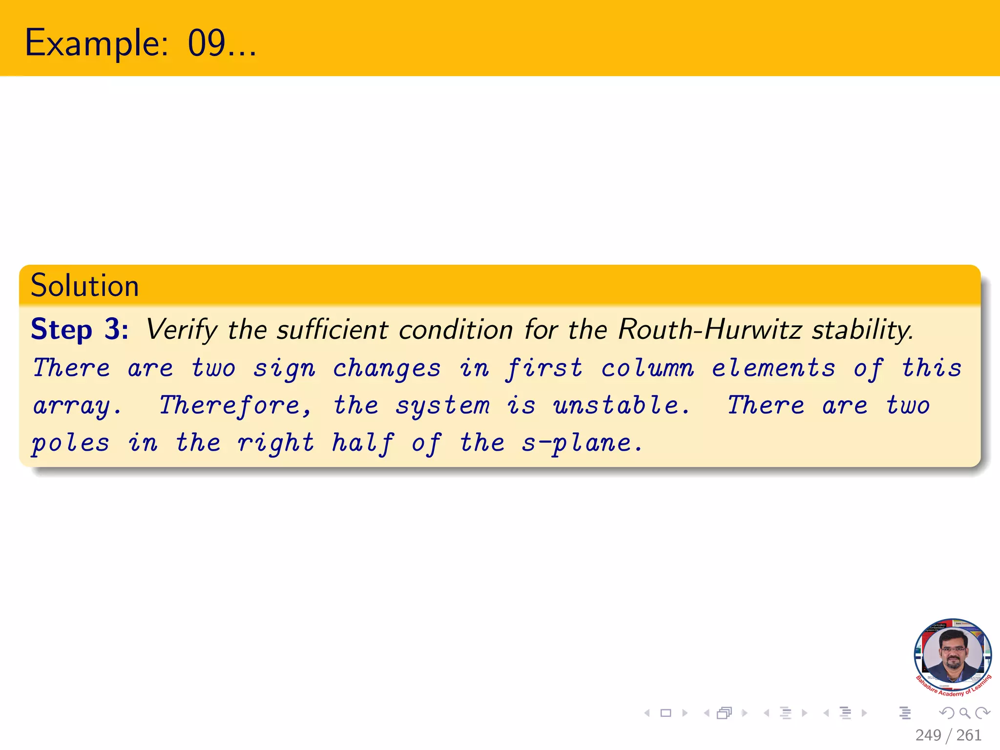
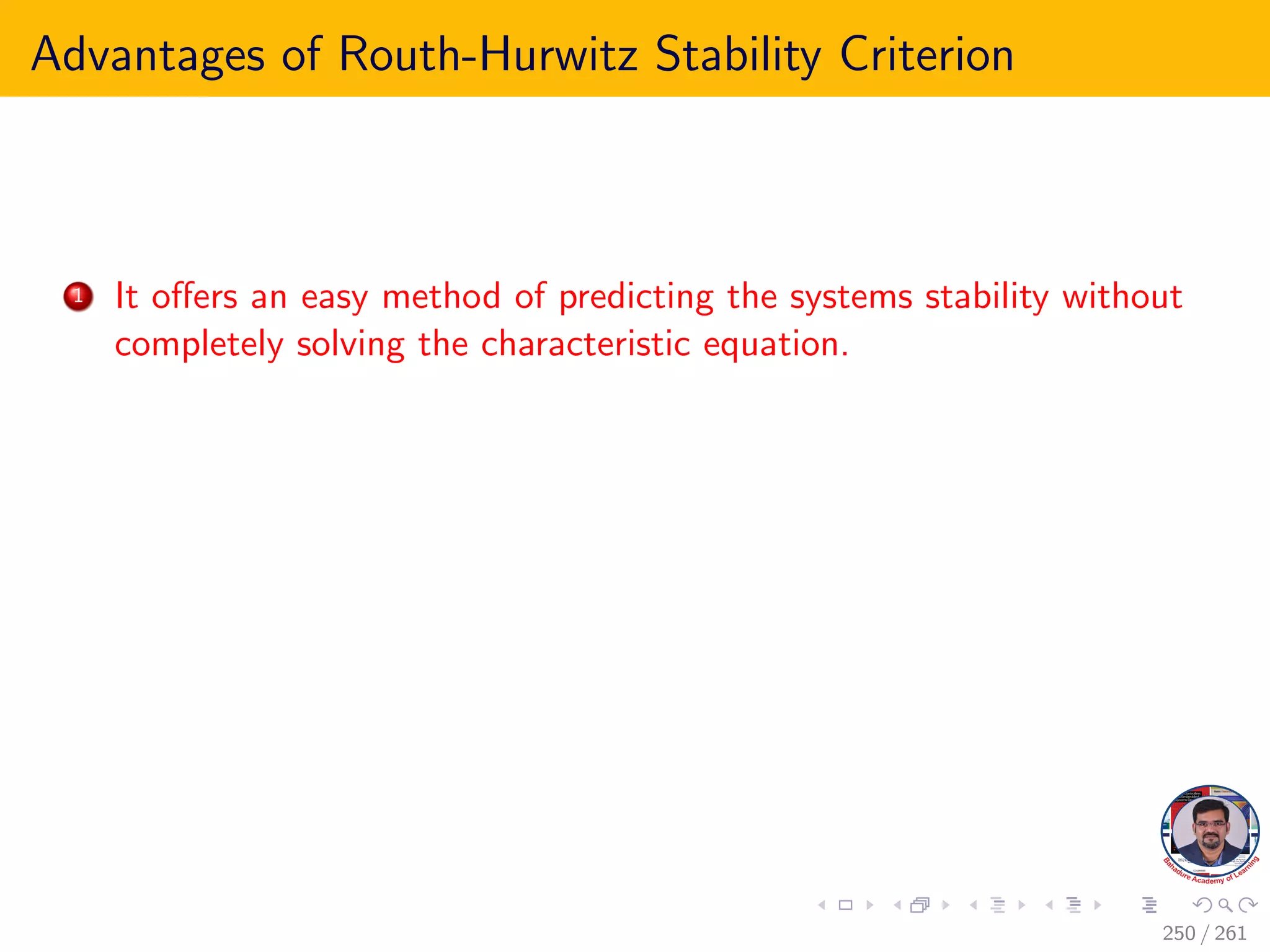
This document explores the stability of control systems, particularly focusing on the Routh-Hurwitz stability criterion, which determines the stability of linear time-invariant systems by analyzing the location of poles in the s-plane. It discusses various types of stability, including absolute, conditional, and marginal stability, and highlights the importance of having poles in specific regions to ensure a stable output. The document outlines the necessary and sufficient conditions for stability as part of the Routh-Hurwitz criterion, emphasizing the significance of coefficient signs and presence in the characteristic equation.

1. Control System
Stability: Routh Criterion
Nilesh Bhaskarrao Bahadure
Ph.D, ME, BE
nbahadure@gmail.com
https://www.sites.google.com/site/nileshbbahadure/home
June 29, 2021
1 / 261

2. Overview I
1 Introduction
2 Types of Stable System
3 Routh-Hurwitz Stability Criterion
Disadvantages of Hurwitz Criterion
Techniques of Routh-Hurwitz criterion
4 Examples
5 Special Cases of Routh Array
6 Advantages and Disadvantages of Routh-Hurwitz Stability Criterion
7 Thank You
2 / 261

3. The Stability of Linear Feedback Systems
3 / 261

4. The Stability of Linear Feedback Systems
The issue of ensuring the stability of a closed-loop feedback system is
central to control system design. Knowing that an unstable closed-loop
system is generally of no practical value, we seek methods to help us
analyze and design stable systems. A stable system should exhibit a
bounded output if the corresponding input is bounded.
4 / 261

5. The Stability of Linear Feedback Systems...
5 / 261

6. The Stability of Linear Feedback Systems...
The stability of a control system is defined as the ability of any system to
provide a bounded output when a bounded input is applied to it. More
specifically, we can say, that stability allows the system to reach the
steady-state and remain in that state for that particular input even after
variation in the parameters of the system.
6 / 261

7. The Stability of Linear Feedback Systems...
The stability of a control system is defined as the ability of any system to
provide a bounded output when a bounded input is applied to it. More
specifically, we can say, that stability allows the system to reach the
steady-state and remain in that state for that particular input even after
variation in the parameters of the system.
Stability is considered to be an important property of a control system. It
is also referred as the systems ability to reach the steady-state.
7 / 261

8. Stability of Control System
8 / 261

9. Stability of Control System
We have already discussed that a stable system generates bounded output
for bounded input (BIBO).
9 / 261

10. Stability of Control System
We have already discussed that a stable system generates bounded output
for bounded input (BIBO).
Now the question arises what is bounded signal?
Bounded value of a signal represents a finite value. More specifically, we
can say, the bounded signal holds a finite value of maxima and minima.
Thus, if maxima and minima of any signal are finite then this means all
the other values between maxima and minima will also be finite.
Suppose we have a signal shown below:
Figure : Bounded signal
10 / 261

11. Stability of Control System...
11 / 261

12. Stability of Control System...
As we can see that here the maxima and minima of the signal represented
above is having finite values. Thus such a signal is said to be bounded and
if such an output is provided by a system then it is said to be a stable
system.
12 / 261

13. Stability of Control System...
As we can see that here the maxima and minima of the signal represented
above is having finite values. Thus such a signal is said to be bounded and
if such an output is provided by a system then it is said to be a stable
system.
Therefore, conversely, we can say that an unstable system provides an
unbounded output when the applied input is bounded in nature.
13 / 261

14. Stability of Control System...
14 / 261

15. Stability of Control System...
Now, what are unbounded signals?
15 / 261

16. Stability of Control System...
Now, what are unbounded signals?
So, generally, the signals whose graph shows continuous rise thereby
showing infinite value such as ramp signal are known as unbounded
signals. The figure shown below represents the unbounded signal:
Figure : Unbounded signal
16 / 261

17. Stability of Control System...
17 / 261

18. Stability of Control System...
Sometimes we come across asymptotically stable systems which are
defined as the systems whose output progresses 0, when the input is not
present, even when the parameters of the system show variation.
18 / 261

19. Stability of Control System...
Sometimes we come across asymptotically stable systems which are
defined as the systems whose output progresses 0, when the input is not
present, even when the parameters of the system show variation.
It is to be noted here that poles of the transfer function, is a factor
defining the stability of the control system.
19 / 261

20. How poles can give information regarding the stability of
the system?
Case I
20 / 261

21. How poles can give information regarding the stability of
the system?
Case I
When the poles of the transfer function of the system are located on the
left side of the s-plane then it is said to be a stable system. However, as
the poles progress towards 0 or origin, then, in this case, the stability of
the system decreases.
21 / 261

22. How poles can give information regarding the stability of
the system?
Case I
When the poles of the transfer function of the system are located on the
left side of the s-plane then it is said to be a stable system. However, as
the poles progress towards 0 or origin, then, in this case, the stability of
the system decreases.
Figure : Poles on left side of the s-plane
22 / 261

23. How poles...
Case II
23 / 261

24. How poles...
Case II
If for a system, the poles are present in the imaginary axis and are
non-repetitive in nature, then it is said to be a marginally stable system.
24 / 261

25. How poles...
Case II
If for a system, the poles are present in the imaginary axis and are
non-repetitive in nature, then it is said to be a marginally stable system.
Figure : Poles on imaginary axis s-plane
25 / 261

26. How poles...
Case III
26 / 261

27. How poles...
Case III
However, if there exist repetitive poles in the imaginary axis of the s-plane.
Then it is called to be an unstable system.
27 / 261

28. How poles...
Case III
However, if there exist repetitive poles in the imaginary axis of the s-plane.
Then it is called to be an unstable system.
Figure : Poles on imaginary axis s-plane
28 / 261

29. How poles...
Case IV
29 / 261

30. How poles...
Case IV
If a system having poles in the right domain of the s-plane, then such a
system is called an unstable system. The presence of even a single pole in
the right half makes the system unstable.
30 / 261

31. How poles...
Case IV
If a system having poles in the right domain of the s-plane, then such a
system is called an unstable system. The presence of even a single pole in
the right half makes the system unstable.
Figure : Poles on right hand side of s-plane
31 / 261

32. Absolutely stable system
Absolutely stable system
32 / 261

33. Absolutely stable system
Absolutely stable system
An absolutely stable system is the one that provides bounded output even
for the variation in the parameters of the system. This means it is such a
system whose output after reaching a steady-state does not show changes
irrespective of the disturbances or variation in the system parameter values.
33 / 261

34. Absolutely stable system
Absolutely stable system
An absolutely stable system is the one that provides bounded output even
for the variation in the parameters of the system. This means it is such a
system whose output after reaching a steady-state does not show changes
irrespective of the disturbances or variation in the system parameter values.
The figure shown below represents the step response of an absolutely
stable system:
34 / 261

35. Absolutely stable system
Absolutely stable system
An absolutely stable system is the one that provides bounded output even
for the variation in the parameters of the system. This means it is such a
system whose output after reaching a steady-state does not show changes
irrespective of the disturbances or variation in the system parameter values.
The figure shown below represents the step response of an absolutely
stable system:
35 / 261

36. Absolutely stable system...
Absolutely stable system...
36 / 261

37. Absolutely stable system...
Absolutely stable system...
The nature of poles for the absolutely stable condition must be real and
negative.
37 / 261

38. Absolutely stable system...
Absolutely stable system...
The nature of poles for the absolutely stable condition must be real and
negative.
The figure below represents an unstable system:
38 / 261

39. Absolutely stable system...
Absolutely stable system...
The nature of poles for the absolutely stable condition must be real and
negative.
The figure below represents an unstable system:
Figure : Unstable system
39 / 261

40. Conditionally stable system
Conditionally stable system
40 / 261

41. Conditionally stable system
Conditionally stable system
A conditionally stable system gives bounded output for the only specific
conditions of the system that is defined by the parameter of the system.
41 / 261

42. Conditionally stable system
Conditionally stable system
A conditionally stable system gives bounded output for the only specific
conditions of the system that is defined by the parameter of the system.
Thus we can say here the system exhibits stability only under particular
conditions.
42 / 261

43. Conditionally stable system
Conditionally stable system
A conditionally stable system gives bounded output for the only specific
conditions of the system that is defined by the parameter of the system.
Thus we can say here the system exhibits stability only under particular
conditions.
And if that particular condition is violated then the system generates
unbounded output.
43 / 261

44. Marginally/ Critically stable system
Marginally/ Critically stable system
44 / 261

45. Marginally/ Critically stable system
Marginally/ Critically stable system
A marginally stable system is the one that generates a signal which is
oscillating with constant frequency and amplitude when a bounded input is
provided to it.
45 / 261

46. Marginally/ Critically stable system
Marginally/ Critically stable system
A marginally stable system is the one that generates a signal which is
oscillating with constant frequency and amplitude when a bounded input is
provided to it.
These oscillations are known as sustained oscillations. The figure here
represents the step response of a marginally stable system:
46 / 261

47. Marginally/ Critically stable system
Marginally/ Critically stable system
A marginally stable system is the one that generates a signal which is
oscillating with constant frequency and amplitude when a bounded input is
provided to it.
These oscillations are known as sustained oscillations. The figure here
represents the step response of a marginally stable system:
Figure : Marginally/ Critically stable system 47 / 261

48. Marginally/ Critically stable system
Marginally/ Critically stable system
A marginally stable system is the one that generates a signal which is
oscillating with constant frequency and amplitude when a bounded input is
provided to it.
These oscillations are known as sustained oscillations. The figure here
represents the step response of a marginally stable system:
Figure : Marginally/ Critically stable system 48 / 261

49. Marginally/ Critically stable system
Marginally/ Critically stable system
A marginally stable system is the one that generates a signal which is
oscillating with constant frequency and amplitude when a bounded input is
provided to it.
These oscillations are known as sustained oscillations. The figure here
represents the step response of a marginally stable system:
Figure : Marginally/ Critically stable system 49 / 261

50. Marginally/ Critically stable system...
50 / 261

51. Marginally/ Critically stable system...
The nature of the closed-loop poles must be non-repetitive and located on
the imaginary axis.
51 / 261

52. Marginally/ Critically stable system...
The nature of the closed-loop poles must be non-repetitive and located on
the imaginary axis.
In this way, the stability of the control system is studied.
52 / 261

53. Routh-Hurwitz Stability Criterion
53 / 261

54. Routh-Hurwitz Stability Criterion
Routh-Hurwitz stability criterion is an analytical method used for the
determination of stability of a linear time-invariant system. The basis of
this criterion revolves around simply determining the location of poles of
the characteristic equation in either left half or right half of s-plane despite
solving the equation.
54 / 261

55. Routh-Hurwitz Stability Criterion
Routh-Hurwitz stability criterion is an analytical method used for the
determination of stability of a linear time-invariant system. The basis of
this criterion revolves around simply determining the location of poles of
the characteristic equation in either left half or right half of s-plane despite
solving the equation.
The stability of a control system basically defines its ability to reach the
steady-state and remain there till the time, specific input is maintained
despite the variation in the other factors associated with the system.
55 / 261

56. Routh-Hurwitz Stability Criterion
Routh-Hurwitz stability criterion is an analytical method used for the
determination of stability of a linear time-invariant system. The basis of
this criterion revolves around simply determining the location of poles of
the characteristic equation in either left half or right half of s-plane despite
solving the equation.
The stability of a control system basically defines its ability to reach the
steady-state and remain there till the time, specific input is maintained
despite the variation in the other factors associated with the system.
Thus, to check whether the system is stable or not, the conditions of
stability criterion must be satisfied.
56 / 261

57. Routh-Hurwitz Criterion
57 / 261

58. Routh-Hurwitz Criterion
This stability criterion is known to be an algebraic technique that uses the
characteristic equation of the transfer function of the closed-loop control
system in order to determine its stability.
58 / 261

59. Routh-Hurwitz Criterion
This stability criterion is known to be an algebraic technique that uses the
characteristic equation of the transfer function of the closed-loop control
system in order to determine its stability.
According to this criterion, there is a necessary condition and a sufficient
condition.
59 / 261

60. Routh-Hurwitz Criterion
This stability criterion is known to be an algebraic technique that uses the
characteristic equation of the transfer function of the closed-loop control
system in order to determine its stability.
According to this criterion, there is a necessary condition and a sufficient
condition.
If the necessary condition is not satisfied by the system, then it is said to
be an unstable system. However, even after satisfying the necessary
condition, the system may or may not be stable.
60 / 261

61. Routh-Hurwitz Criterion
This stability criterion is known to be an algebraic technique that uses the
characteristic equation of the transfer function of the closed-loop control
system in order to determine its stability.
According to this criterion, there is a necessary condition and a sufficient
condition.
If the necessary condition is not satisfied by the system, then it is said to
be an unstable system. However, even after satisfying the necessary
condition, the system may or may not be stable.
Therefore, we need sufficient condition to determine whether the system is
stable or not.
61 / 261

62. Routh-Hurwitz Criterion...
62 / 261

63. Routh-Hurwitz Criterion...
Suppose the transfer function of the closed-loop system is given as:
C(s)
R(s)
=
b0sm + b1sm−1 + − − − + bm
a0sn + a1sn−1 + − − − + an
=
B(s)
F(s)
where a and b are the two constants here.
63 / 261

64. Routh-Hurwitz Criterion...
Suppose the transfer function of the closed-loop system is given as:
C(s)
R(s)
=
b0sm + b1sm−1 + − − − + bm
a0sn + a1sn−1 + − − − + an
=
B(s)
F(s)
where a and b are the two constants here.
On equating F(s) = 0, we will get the closed-loop poles of the system,
which is known as the characteristic equation of the system, given as:
F(s) = a0sn
+ a1sn−1
+ a2sn−2
+ − − − + an
= 0
64 / 261

65. Routh-Hurwitz Criterion...
65 / 261

66. Routh-Hurwitz Criterion...
Moreover, the roots of this characteristic equation are the poles of the
system with the help of which the stability of the system is decided.
66 / 261

67. Routh-Hurwitz Criterion...
Moreover, the roots of this characteristic equation are the poles of the
system with the help of which the stability of the system is decided.
It is to be noted here that before checking the stability of the system using
the Routh-Hurwitz criterion, a basic analysis must be done.
67 / 261

68. Routh-Hurwitz Criterion...
Moreover, the roots of this characteristic equation are the poles of the
system with the help of which the stability of the system is decided.
It is to be noted here that before checking the stability of the system using
the Routh-Hurwitz criterion, a basic analysis must be done.
This general test is simply done by analyzing the characteristic equation,
here all the roots of the equation must be present on the left side of the
s-plane.
68 / 261

69. Routh-Hurwitz Criterion...
The necessary conditions are discussed below:
1 The coefficients of all the polynomials of the equation should be of a
similar sign.
69 / 261

70. Routh-Hurwitz Criterion...
The necessary conditions are discussed below:
1 The coefficients of all the polynomials of the equation should be of a
similar sign.
2 Also, all the coefficients must be present, this means that any of the
power of ’s’ from ’n’ to 0 must not be absent.
70 / 261

71. Routh-Hurwitz Criterion...
The necessary conditions are discussed below:
1 The coefficients of all the polynomials of the equation should be of a
similar sign.
2 Also, all the coefficients must be present, this means that any of the
power of ’s’ from ’n’ to 0 must not be absent.
71 / 261

72. Routh-Hurwitz Criterion...
The necessary conditions are discussed below:
1 The coefficients of all the polynomials of the equation should be of a
similar sign.
2 Also, all the coefficients must be present, this means that any of the
power of ’s’ from ’n’ to 0 must not be absent.
These two are not sufficient conditions to prove the stability of the system.
72 / 261

73. Routh-Hurwitz Criterion...
The necessary conditions are discussed below:
1 The coefficients of all the polynomials of the equation should be of a
similar sign.
2 Also, all the coefficients must be present, this means that any of the
power of ’s’ from ’n’ to 0 must not be absent.
These two are not sufficient conditions to prove the stability of the system.
Initially, the sufficient condition to have the poles in the left half of s-plane
was proposed by Hurwitz. It was known as Hurwitz criterion and states
that all the subdeterminants of the Hurwitz’s determinant must be
positive.
73 / 261

74. Disadvantages of Hurwitz Criterion
Disadvantages:
1 Solving the determinants of the higher-order system is quite difficult
and time-consuming.
74 / 261

75. Disadvantages of Hurwitz Criterion
Disadvantages:
1 Solving the determinants of the higher-order system is quite difficult
and time-consuming.
2 In the case of an unstable system, the number of roots in the right
half of s-plane is non-determinable by this method.
75 / 261

76. Disadvantages of Hurwitz Criterion
Disadvantages:
1 Solving the determinants of the higher-order system is quite difficult
and time-consuming.
2 In the case of an unstable system, the number of roots in the right
half of s-plane is non-determinable by this method.
3 The prediction of marginal stability is not easy.
76 / 261

77. Disadvantages of Hurwitz Criterion
Disadvantages:
1 Solving the determinants of the higher-order system is quite difficult
and time-consuming.
2 In the case of an unstable system, the number of roots in the right
half of s-plane is non-determinable by this method.
3 The prediction of marginal stability is not easy.
77 / 261

78. Disadvantages of Hurwitz Criterion
Disadvantages:
1 Solving the determinants of the higher-order system is quite difficult
and time-consuming.
2 In the case of an unstable system, the number of roots in the right
half of s-plane is non-determinable by this method.
3 The prediction of marginal stability is not easy.
So, because of these disadvantages, Routh proposed another technique for
determining the stability of the system, this method is generally known as
the Routh-Hurwitz criterion or Routh’s criterion.
78 / 261

79. Techniques of Routh-Hurwitz criterion
79 / 261

80. Techniques of Routh-Hurwitz criterion
According to Routh, for a stable system the necessary and sufficient
condition is that in a routh array, all the terms that are present in the first
column must be of the similar sign. This means no change of sign (either
from positive to negative or negative to positive) must exist in the first
column of the array.
80 / 261

81. Techniques of Routh-Hurwitz criterion
According to Routh, for a stable system the necessary and sufficient
condition is that in a routh array, all the terms that are present in the first
column must be of the similar sign. This means no change of sign (either
from positive to negative or negative to positive) must exist in the first
column of the array.
Therefore, in case if there is any sign change then such a system becomes
unstable.
81 / 261

82. Techniques of Routh-Hurwitz criterion
According to Routh, for a stable system the necessary and sufficient
condition is that in a routh array, all the terms that are present in the first
column must be of the similar sign. This means no change of sign (either
from positive to negative or negative to positive) must exist in the first
column of the array.
Therefore, in case if there is any sign change then such a system becomes
unstable.
This is said on the basis that the overall sign changes in the first column
signify the total number of roots lying on the right half of the s-plane,
thereby making the system unstable.
82 / 261

83. Techniques of Routh-Hurwitz criterion
According to Routh, for a stable system the necessary and sufficient
condition is that in a routh array, all the terms that are present in the first
column must be of the similar sign. This means no change of sign (either
from positive to negative or negative to positive) must exist in the first
column of the array.
Therefore, in case if there is any sign change then such a system becomes
unstable.
This is said on the basis that the overall sign changes in the first column
signify the total number of roots lying on the right half of the s-plane,
thereby making the system unstable.
Thus, in simple words, we can say, that for a system to be stable, each
coefficient of the first column of the array must have a positive sign. If it
is not so, then it is an unstable system. And the number of sign change
that makes the system unstable shows the number of poles that are
present on the right side of the s-plane.
83 / 261

84. Techniques of Routh-Hurwitz criterion
According to Routh, for a stable system the necessary and sufficient
condition is that in a routh array, all the terms that are present in the first
column must be of the similar sign. This means no change of sign (either
from positive to negative or negative to positive) must exist in the first
column of the array.
Therefore, in case if there is any sign change then such a system becomes
unstable.
This is said on the basis that the overall sign changes in the first column
signify the total number of roots lying on the right half of the s-plane,
thereby making the system unstable.
Thus, in simple words, we can say, that for a system to be stable, each
coefficient of the first column of the array must have a positive sign. If it
is not so, then it is an unstable system. And the number of sign change
that makes the system unstable shows the number of poles that are
present on the right side of the s-plane.
This is known as the Routh-Hurwitz Criterion.
84 / 261

85. What is Routh Array?
85 / 261

86. What is Routh Array?
Basically, under the Routh-Hurwitz stability criterion, Routh proposed a
technique by which the coefficients of the characteristic equation are
arranged in a specific manner. This arrangement of the coefficients forms
an array which is known as routh array.
86 / 261

87. What is Routh Array?
Basically, under the Routh-Hurwitz stability criterion, Routh proposed a
technique by which the coefficients of the characteristic equation are
arranged in a specific manner. This arrangement of the coefficients forms
an array which is known as routh array.
Let us now see how a routh array is formed. Consider the general
characteristic equation:
F(s) = a0sn
+ a1sn−1
+ a2sn−2
+ − − − + an
= 0
87 / 261

88. What is Routh Array?
Basically, under the Routh-Hurwitz stability criterion, Routh proposed a
technique by which the coefficients of the characteristic equation are
arranged in a specific manner. This arrangement of the coefficients forms
an array which is known as routh array.
Let us now see how a routh array is formed. Consider the general
characteristic equation:
F(s) = a0sn
+ a1sn−1
+ a2sn−2
+ − − − + an
= 0
For the routh array, the first two rows are written from the characteristic
equation directly while the rest of the rows are formed with the help of
previous rows.
88 / 261

89. What is Routh Array?
Basically, under the Routh-Hurwitz stability criterion, Routh proposed a
technique by which the coefficients of the characteristic equation are
arranged in a specific manner. This arrangement of the coefficients forms
an array which is known as routh array.
Let us now see how a routh array is formed. Consider the general
characteristic equation:
F(s) = a0sn
+ a1sn−1
+ a2sn−2
+ − − − + an
= 0
For the routh array, the first two rows are written from the characteristic
equation directly while the rest of the rows are formed with the help of
previous rows.
It is to be noted here that if in the characteristic equation, n is odd
then the first row of the array will hold the odd coefficients. While if
n is even then there will be even coefficients present in the first row.
89 / 261

90. What is Routh Array?
Basically, under the Routh-Hurwitz stability criterion, Routh proposed a
technique by which the coefficients of the characteristic equation are
arranged in a specific manner. This arrangement of the coefficients forms
an array which is known as routh array.
Let us now see how a routh array is formed. Consider the general
characteristic equation:
F(s) = a0sn
+ a1sn−1
+ a2sn−2
+ − − − + an
= 0
For the routh array, the first two rows are written from the characteristic
equation directly while the rest of the rows are formed with the help of
previous rows.
It is to be noted here that if in the characteristic equation, n is odd
then the first row of the array will hold the odd coefficients. While if
n is even then there will be even coefficients present in the first row.
In this way, the first and second row of the array will get formed. Let us
now see how the rest of the rows will get formed.
90 / 261

91. What is Routh Array?...
91 / 261

92. What is Routh Array?...
Figure : Routh Array
92 / 261

93. What is Routh Array?...
93 / 261

94. What is Routh Array?...
So, the third row will be formed using the first and second rows. Let us
see how
94 / 261

95. What is Routh Array?...
So, the third row will be formed using the first and second rows. Let us
see how
b1 =
a1a2 − a0a3
a1
,
95 / 261

96. What is Routh Array?...
So, the third row will be formed using the first and second rows. Let us
see how
b1 =
a1a2 − a0a3
a1
, b2 =
a1a4 − a0a5
a1
,
96 / 261

97. What is Routh Array?...
So, the third row will be formed using the first and second rows. Let us
see how
b1 =
a1a2 − a0a3
a1
, b2 =
a1a4 − a0a5
a1
, b3 =
a1a6 − a0a7
a1
− −−
In a similar way after forming the 3rd row, we can use 2nd and 3rd row to
form the 4th row
97 / 261

98. What is Routh Array?...
So, the third row will be formed using the first and second rows. Let us
see how
b1 =
a1a2 − a0a3
a1
, b2 =
a1a4 − a0a5
a1
, b3 =
a1a6 − a0a7
a1
− −−
In a similar way after forming the 3rd row, we can use 2nd and 3rd row to
form the 4th row
c1 =
b1a3 − a1b2
b1
,
98 / 261

99. What is Routh Array?...
So, the third row will be formed using the first and second rows. Let us
see how
b1 =
a1a2 − a0a3
a1
, b2 =
a1a4 − a0a5
a1
, b3 =
a1a6 − a0a7
a1
− −−
In a similar way after forming the 3rd row, we can use 2nd and 3rd row to
form the 4th row
c1 =
b1a3 − a1b2
b1
, c2 =
b1a5 − a1b3
b1
,
99 / 261

100. What is Routh Array?...
So, the third row will be formed using the first and second rows. Let us
see how
b1 =
a1a2 − a0a3
a1
, b2 =
a1a4 − a0a5
a1
, b3 =
a1a6 − a0a7
a1
− −−
In a similar way after forming the 3rd row, we can use 2nd and 3rd row to
form the 4th row
c1 =
b1a3 − a1b2
b1
, c2 =
b1a5 − a1b3
b1
, c3 =
b1a6 − a1b4
b1
− −−
and so on.
100 / 261

101. What is Routh Array?...
So, the third row will be formed using the first and second rows. Let us
see how
b1 =
a1a2 − a0a3
a1
, b2 =
a1a4 − a0a5
a1
, b3 =
a1a6 − a0a7
a1
− −−
In a similar way after forming the 3rd row, we can use 2nd and 3rd row to
form the 4th row
c1 =
b1a3 − a1b2
b1
, c2 =
b1a5 − a1b3
b1
, c3 =
b1a6 − a1b4
b1
− −−
and so on.
Therefore, we have to continue the process until the time we get the
coefficients for s0, which is nothing but an. In this way, we get routh array
from which the stability of the system is predicted.
101 / 261

102. What is Routh Array?...
So, the third row will be formed using the first and second rows. Let us
see how
b1 =
a1a2 − a0a3
a1
, b2 =
a1a4 − a0a5
a1
, b3 =
a1a6 − a0a7
a1
− −−
In a similar way after forming the 3rd row, we can use 2nd and 3rd row to
form the 4th row
c1 =
b1a3 − a1b2
b1
, c2 =
b1a5 − a1b3
b1
, c3 =
b1a6 − a1b4
b1
− −−
and so on.
Therefore, we have to continue the process until the time we get the
coefficients for s0, which is nothing but an. In this way, we get routh array
from which the stability of the system is predicted.
Now there are two special cases that cause the failure of the Routh’s test:
102 / 261

103. Two special cases that cause the failure of the Routh’s test
Case 1:
103 / 261

104. Two special cases that cause the failure of the Routh’s test
Case 1:
If in any of the rows the first element is 0 and in the same row even a
single non zero element is there then in the next row there will be an
infinite term and this will lead to failure of Routh’s test.
Case 2:
104 / 261

105. Two special cases that cause the failure of the Routh’s test
Case 1:
If in any of the rows the first element is 0 and in the same row even a
single non zero element is there then in the next row there will be an
infinite term and this will lead to failure of Routh’s test.
Case 2:
If there is such a row in routh array whose all the elements are 0 then it
will be impossible to determine the next row and thus the Routh’s test
fails in this condition also. This is so because the presence of only 0 in a
row shows the absence of coefficients in that particular row.
105 / 261

106. Example: 01
Example
106 / 261

107. Example: 01
Example
find the stability of the control system having characteristic equation,
s4
+ 3s3
+ 3s2
+ 2s + 1 = 0
107 / 261

108. Example: 01
Solution
108 / 261

109. Example: 01
Solution
Step 1: Verify the necessary condition for the Routh-Hurwitz stability.
All the coefficients of the characteristic polynomial, s4 + 3s3 + 3s2 + 2s + 1
are positive. So, the control system satisfies the necessary condition.
109 / 261

110. Example: 01
Solution
Step 1: Verify the necessary condition for the Routh-Hurwitz stability.
All the coefficients of the characteristic polynomial, s4 + 3s3 + 3s2 + 2s + 1
are positive. So, the control system satisfies the necessary condition.
Step 2: Form the Routh array for the given characteristic polynomial.
110 / 261

111. Example: 01
Solution
Step 1: Verify the necessary condition for the Routh-Hurwitz stability.
All the coefficients of the characteristic polynomial, s4 + 3s3 + 3s2 + 2s + 1
are positive. So, the control system satisfies the necessary condition.
Step 2: Form the Routh array for the given characteristic polynomial.
s4 1 3 1
111 / 261

112. Example: 01
Solution
Step 1: Verify the necessary condition for the Routh-Hurwitz stability.
All the coefficients of the characteristic polynomial, s4 + 3s3 + 3s2 + 2s + 1
are positive. So, the control system satisfies the necessary condition.
Step 2: Form the Routh array for the given characteristic polynomial.
s4 1 3 1
s3 3 2
112 / 261

113. Example: 01
Solution
Step 1: Verify the necessary condition for the Routh-Hurwitz stability.
All the coefficients of the characteristic polynomial, s4 + 3s3 + 3s2 + 2s + 1
are positive. So, the control system satisfies the necessary condition.
Step 2: Form the Routh array for the given characteristic polynomial.
s4 1 3 1
s3 3 2
s2 (3∗3)−(2∗1)
3 = 7
3
(3∗1)−(0∗1)
3 = 1
113 / 261

114. Example: 01
Solution
Step 1: Verify the necessary condition for the Routh-Hurwitz stability.
All the coefficients of the characteristic polynomial, s4 + 3s3 + 3s2 + 2s + 1
are positive. So, the control system satisfies the necessary condition.
Step 2: Form the Routh array for the given characteristic polynomial.
s4 1 3 1
s3 3 2
s2 (3∗3)−(2∗1)
3 = 7
3
(3∗1)−(0∗1)
3 = 1
s1 ( 7
3
∗2)−(1∗3)
7
3
= 5
7
114 / 261

115. Example: 01
Solution
Step 1: Verify the necessary condition for the Routh-Hurwitz stability.
All the coefficients of the characteristic polynomial, s4 + 3s3 + 3s2 + 2s + 1
are positive. So, the control system satisfies the necessary condition.
Step 2: Form the Routh array for the given characteristic polynomial.
s4 1 3 1
s3 3 2
s2 (3∗3)−(2∗1)
3 = 7
3
(3∗1)−(0∗1)
3 = 1
s1 ( 7
3
∗2)−(1∗3)
7
3
= 5
7
s0 1
115 / 261

116. Example: 01
Solution
Step 1: Verify the necessary condition for the Routh-Hurwitz stability.
All the coefficients of the characteristic polynomial, s4 + 3s3 + 3s2 + 2s + 1
are positive. So, the control system satisfies the necessary condition.
Step 2: Form the Routh array for the given characteristic polynomial.
s4 1 3 1
s3 3 2
s2 (3∗3)−(2∗1)
3 = 7
3
(3∗1)−(0∗1)
3 = 1
s1 ( 7
3
∗2)−(1∗3)
7
3
= 5
7
s0 1
Step 3: Verify the sufficient condition for the Routh-Hurwitz stability.
All the elements of the first column of the Routh array are
positive. There is no sign change in the first column of
the Routh array. So, the control system is stable.
116 / 261

117. Example: 02
Example
117 / 261

118. Example: 02
Example
Check the stability of the system whose characteristic equation is given by
s4
+ 2s3
+ 6s2
+ 4s + 1 = 0
118 / 261

119. Example: 02
Solution
119 / 261

120. Example: 02
Solution
Step 1: Verify the necessary condition for the Routh-Hurwitz stability.
All the coefficients of the characteristic polynomial,
s4 + 2s3 + 6s2 + 4s + 1 = 0 are positive. So, the control system satisfies
the necessary condition.
120 / 261

121. Example: 02
Solution
Step 1: Verify the necessary condition for the Routh-Hurwitz stability.
All the coefficients of the characteristic polynomial,
s4 + 2s3 + 6s2 + 4s + 1 = 0 are positive. So, the control system satisfies
the necessary condition.
Step 2: Form the Routh array for the given characteristic polynomial.
121 / 261

122. Example: 02
Solution
Step 1: Verify the necessary condition for the Routh-Hurwitz stability.
All the coefficients of the characteristic polynomial,
s4 + 2s3 + 6s2 + 4s + 1 = 0 are positive. So, the control system satisfies
the necessary condition.
Step 2: Form the Routh array for the given characteristic polynomial.
s4 1 6 1
122 / 261

123. Example: 02
Solution
Step 1: Verify the necessary condition for the Routh-Hurwitz stability.
All the coefficients of the characteristic polynomial,
s4 + 2s3 + 6s2 + 4s + 1 = 0 are positive. So, the control system satisfies
the necessary condition.
Step 2: Form the Routh array for the given characteristic polynomial.
s4 1 6 1
s3 2 4
123 / 261

124. Example: 02
Solution
Step 1: Verify the necessary condition for the Routh-Hurwitz stability.
All the coefficients of the characteristic polynomial,
s4 + 2s3 + 6s2 + 4s + 1 = 0 are positive. So, the control system satisfies
the necessary condition.
Step 2: Form the Routh array for the given characteristic polynomial.
s4 1 6 1
s3 2 4
s2 (2∗6)−(4∗1)
2 = 4 (2∗1)−(0∗1)
2 = 1
124 / 261

125. Example: 02
Solution
Step 1: Verify the necessary condition for the Routh-Hurwitz stability.
All the coefficients of the characteristic polynomial,
s4 + 2s3 + 6s2 + 4s + 1 = 0 are positive. So, the control system satisfies
the necessary condition.
Step 2: Form the Routh array for the given characteristic polynomial.
s4 1 6 1
s3 2 4
s2 (2∗6)−(4∗1)
2 = 4 (2∗1)−(0∗1)
2 = 1
s1 (4∗4)−(1∗2)
4 = 3.5
125 / 261

126. Example: 02
Solution
Step 1: Verify the necessary condition for the Routh-Hurwitz stability.
All the coefficients of the characteristic polynomial,
s4 + 2s3 + 6s2 + 4s + 1 = 0 are positive. So, the control system satisfies
the necessary condition.
Step 2: Form the Routh array for the given characteristic polynomial.
s4 1 6 1
s3 2 4
s2 (2∗6)−(4∗1)
2 = 4 (2∗1)−(0∗1)
2 = 1
s1 (4∗4)−(1∗2)
4 = 3.5
s0 1
126 / 261

127. Example: 02
Solution
Step 1: Verify the necessary condition for the Routh-Hurwitz stability.
All the coefficients of the characteristic polynomial,
s4 + 2s3 + 6s2 + 4s + 1 = 0 are positive. So, the control system satisfies
the necessary condition.
Step 2: Form the Routh array for the given characteristic polynomial.
s4 1 6 1
s3 2 4
s2 (2∗6)−(4∗1)
2 = 4 (2∗1)−(0∗1)
2 = 1
s1 (4∗4)−(1∗2)
4 = 3.5
s0 1
Step 3: Verify the sufficient condition for the Routh-Hurwitz stability.
Since all the coefficients in the first column are of the
same sign, i.e., positive, the given equation has no roots
with positive real parts; therefore, the system is said to
127 / 261

128. Example: 03
Example
128 / 261

129. Example: 03
Example
Find stability of the following system given by G(s) = K
s(s+1) and H(s) = 1
using Routh-Hurwitz stability criterion.
129 / 261

130. Example: 03
Solution
130 / 261

131. Example: 03
Solution
In the system T(s) = G(s)
1+G(s)H(s) =
K
s(s+1)
1+ K
s(s+1)
Characteristics equation
B(s) = s2
+ s + K = 0
131 / 261

132. Example: 03
Solution
In the system T(s) = G(s)
1+G(s)H(s) =
K
s(s+1)
1+ K
s(s+1)
Characteristics equation
B(s) = s2
+ s + K = 0
Step 1: Verify the necessary condition for the Routh-Hurwitz stability.
All the coefficients of the characteristic polynomial,
B(s) = s2 + s + K = 0 are positive. So, the control system satisfies the
necessary condition (Assuming K > 0).
132 / 261

133. Example: 03
Solution
In the system T(s) = G(s)
1+G(s)H(s) =
K
s(s+1)
1+ K
s(s+1)
Characteristics equation
B(s) = s2
+ s + K = 0
Step 1: Verify the necessary condition for the Routh-Hurwitz stability.
All the coefficients of the characteristic polynomial,
B(s) = s2 + s + K = 0 are positive. So, the control system satisfies the
necessary condition (Assuming K > 0).
Step 2: Form the Routh array for the given characteristic polynomial.
133 / 261

134. Example: 03
Solution
In the system T(s) = G(s)
1+G(s)H(s) =
K
s(s+1)
1+ K
s(s+1)
Characteristics equation
B(s) = s2
+ s + K = 0
Step 1: Verify the necessary condition for the Routh-Hurwitz stability.
All the coefficients of the characteristic polynomial,
B(s) = s2 + s + K = 0 are positive. So, the control system satisfies the
necessary condition (Assuming K > 0).
Step 2: Form the Routh array for the given characteristic polynomial.
s2 1 K
134 / 261

135. Example: 03
Solution
In the system T(s) = G(s)
1+G(s)H(s) =
K
s(s+1)
1+ K
s(s+1)
Characteristics equation
B(s) = s2
+ s + K = 0
Step 1: Verify the necessary condition for the Routh-Hurwitz stability.
All the coefficients of the characteristic polynomial,
B(s) = s2 + s + K = 0 are positive. So, the control system satisfies the
necessary condition (Assuming K > 0).
Step 2: Form the Routh array for the given characteristic polynomial.
s2 1 K
s1 1 0
135 / 261

136. Example: 03
Solution
In the system T(s) = G(s)
1+G(s)H(s) =
K
s(s+1)
1+ K
s(s+1)
Characteristics equation
B(s) = s2
+ s + K = 0
Step 1: Verify the necessary condition for the Routh-Hurwitz stability.
All the coefficients of the characteristic polynomial,
B(s) = s2 + s + K = 0 are positive. So, the control system satisfies the
necessary condition (Assuming K > 0).
Step 2: Form the Routh array for the given characteristic polynomial.
s2 1 K
s1 1 0
s0 K
136 / 261

137. Example: 03...
Solution
137 / 261

138. Example: 03...
Solution
Step 3: Verify the sufficient condition for the Routh-Hurwitz stability.
There are no sign changes in first column elements of this
array.Therefore, the system is always stable for K > 0.
138 / 261

139. Videos on LaTeX, CorelDraw and Many More
139 / 261

140. Example: 04
Example
140 / 261

141. Example: 04
Example
Find stability of the following system given by G(s) = K
s(s+2)(s+4) and
H(s) = 1 using Routh-Hurwitz stability criterion.
141 / 261

142. Example: 04
Solution
142 / 261

143. Example: 04
Solution
In the system T(s) = G(s)
1+G(s)H(s) =
K
s(s+2)(s+4)
1+ K
s(s+2)(s+4)
Characteristics equation
B(s) = s3
+ 6s2
+ 8s + K = 0
143 / 261

144. Example: 04
Solution
In the system T(s) = G(s)
1+G(s)H(s) =
K
s(s+2)(s+4)
1+ K
s(s+2)(s+4)
Characteristics equation
B(s) = s3
+ 6s2
+ 8s + K = 0
Step 1: Verify the necessary condition for the Routh-Hurwitz stability.
All the coefficients of the characteristic polynomial,
B(s) = s3 + 6s2 + 8s + K = 0 are positive. So, the control system
satisfies the necessary condition (Assuming K > 0).
144 / 261

145. Example: 04
Solution
In the system T(s) = G(s)
1+G(s)H(s) =
K
s(s+2)(s+4)
1+ K
s(s+2)(s+4)
Characteristics equation
B(s) = s3
+ 6s2
+ 8s + K = 0
Step 1: Verify the necessary condition for the Routh-Hurwitz stability.
All the coefficients of the characteristic polynomial,
B(s) = s3 + 6s2 + 8s + K = 0 are positive. So, the control system
satisfies the necessary condition (Assuming K > 0).
Step 2: Form the Routh array for the given characteristic polynomial.
145 / 261

146. Example: 04
Solution
In the system T(s) = G(s)
1+G(s)H(s) =
K
s(s+2)(s+4)
1+ K
s(s+2)(s+4)
Characteristics equation
B(s) = s3
+ 6s2
+ 8s + K = 0
Step 1: Verify the necessary condition for the Routh-Hurwitz stability.
All the coefficients of the characteristic polynomial,
B(s) = s3 + 6s2 + 8s + K = 0 are positive. So, the control system
satisfies the necessary condition (Assuming K > 0).
Step 2: Form the Routh array for the given characteristic polynomial.
s3 1 8
146 / 261

147. Example: 04
Solution
In the system T(s) = G(s)
1+G(s)H(s) =
K
s(s+2)(s+4)
1+ K
s(s+2)(s+4)
Characteristics equation
B(s) = s3
+ 6s2
+ 8s + K = 0
Step 1: Verify the necessary condition for the Routh-Hurwitz stability.
All the coefficients of the characteristic polynomial,
B(s) = s3 + 6s2 + 8s + K = 0 are positive. So, the control system
satisfies the necessary condition (Assuming K > 0).
Step 2: Form the Routh array for the given characteristic polynomial.
s3 1 8
s2 6 K
147 / 261

148. Example: 04
Solution
In the system T(s) = G(s)
1+G(s)H(s) =
K
s(s+2)(s+4)
1+ K
s(s+2)(s+4)
Characteristics equation
B(s) = s3
+ 6s2
+ 8s + K = 0
Step 1: Verify the necessary condition for the Routh-Hurwitz stability.
All the coefficients of the characteristic polynomial,
B(s) = s3 + 6s2 + 8s + K = 0 are positive. So, the control system
satisfies the necessary condition (Assuming K > 0).
Step 2: Form the Routh array for the given characteristic polynomial.
s3 1 8
s2 6 K
s1 48−K
6 0
148 / 261

149. Example: 04
Solution
In the system T(s) = G(s)
1+G(s)H(s) =
K
s(s+2)(s+4)
1+ K
s(s+2)(s+4)
Characteristics equation
B(s) = s3
+ 6s2
+ 8s + K = 0
Step 1: Verify the necessary condition for the Routh-Hurwitz stability.
All the coefficients of the characteristic polynomial,
B(s) = s3 + 6s2 + 8s + K = 0 are positive. So, the control system
satisfies the necessary condition (Assuming K > 0).
Step 2: Form the Routh array for the given characteristic polynomial.
s3 1 8
s2 6 K
s1 48−K
6 0
s0 K
149 / 261

150. Example: 04...
Solution
150 / 261

151. Example: 04...
Solution
Step 3: Verify the sufficient condition for the Routh-Hurwitz stability.
151 / 261

152. Example: 04...
Solution
Step 3: Verify the sufficient condition for the Routh-Hurwitz stability.
There are no sign changes in first column elements of this
array if K < 48. Therefore, the system is always stable
for 0 < K < 48
152 / 261

153. Example: 05
Example
153 / 261

154. Example: 05
Example
Find stability of the following system given by B(s) = s3 + 5s2 + 10s + 3
using Routh-Hurwitz stability criterion.
154 / 261

155. Example: 05
Solution
155 / 261

156. Example: 05
Solution
Step 1: Verify the necessary condition for the Routh-Hurwitz stability.
All the coefficients of the characteristic polynomial,
B(s) = s3 + 5s2 + 10s + 3 = 0 are positive. So, the control system
satisfies the necessary condition.
156 / 261

157. Example: 05
Solution
Step 1: Verify the necessary condition for the Routh-Hurwitz stability.
All the coefficients of the characteristic polynomial,
B(s) = s3 + 5s2 + 10s + 3 = 0 are positive. So, the control system
satisfies the necessary condition.
Step 2: Form the Routh array for the given characteristic polynomial.
157 / 261

158. Example: 05
Solution
Step 1: Verify the necessary condition for the Routh-Hurwitz stability.
All the coefficients of the characteristic polynomial,
B(s) = s3 + 5s2 + 10s + 3 = 0 are positive. So, the control system
satisfies the necessary condition.
Step 2: Form the Routh array for the given characteristic polynomial.
s3 1 10
158 / 261

159. Example: 05
Solution
Step 1: Verify the necessary condition for the Routh-Hurwitz stability.
All the coefficients of the characteristic polynomial,
B(s) = s3 + 5s2 + 10s + 3 = 0 are positive. So, the control system
satisfies the necessary condition.
Step 2: Form the Routh array for the given characteristic polynomial.
s3 1 10
s2 5 3
159 / 261

160. Example: 05
Solution
Step 1: Verify the necessary condition for the Routh-Hurwitz stability.
All the coefficients of the characteristic polynomial,
B(s) = s3 + 5s2 + 10s + 3 = 0 are positive. So, the control system
satisfies the necessary condition.
Step 2: Form the Routh array for the given characteristic polynomial.
s3 1 10
s2 5 3
s1 50−3
5 = 9.4 0
160 / 261

161. Example: 05
Solution
Step 1: Verify the necessary condition for the Routh-Hurwitz stability.
All the coefficients of the characteristic polynomial,
B(s) = s3 + 5s2 + 10s + 3 = 0 are positive. So, the control system
satisfies the necessary condition.
Step 2: Form the Routh array for the given characteristic polynomial.
s3 1 10
s2 5 3
s1 50−3
5 = 9.4 0
s0 3
161 / 261

162. Example: 05...
Solution
162 / 261

163. Example: 05...
Solution
Step 3: Verify the sufficient condition for the Routh-Hurwitz stability.
There are no sign changes in first column elements of this
array. Therefore, the system is always stable.
163 / 261

164. Do it by yourself
164 / 261

165. Example: 06
Example
165 / 261

166. Example: 06
Example
Find stability of the following system given by B(s) = s3 + 2s2 + 3s + 10
using Routh-Hurwitz stability criterion.
166 / 261

167. Example: 06
Solution
167 / 261

168. Example: 06
Solution
Step 1: Verify the necessary condition for the Routh-Hurwitz stability.
All the coefficients of the characteristic polynomial,
B(s) = s3 + 2s2 + 3s + 10 = 0 are positive. So, the control system
satisfies the necessary condition.
168 / 261

169. Example: 06
Solution
Step 1: Verify the necessary condition for the Routh-Hurwitz stability.
All the coefficients of the characteristic polynomial,
B(s) = s3 + 2s2 + 3s + 10 = 0 are positive. So, the control system
satisfies the necessary condition.
Step 2: Form the Routh array for the given characteristic polynomial.
169 / 261

170. Example: 06
Solution
Step 1: Verify the necessary condition for the Routh-Hurwitz stability.
All the coefficients of the characteristic polynomial,
B(s) = s3 + 2s2 + 3s + 10 = 0 are positive. So, the control system
satisfies the necessary condition.
Step 2: Form the Routh array for the given characteristic polynomial.
s3 1 3
170 / 261

171. Example: 06
Solution
Step 1: Verify the necessary condition for the Routh-Hurwitz stability.
All the coefficients of the characteristic polynomial,
B(s) = s3 + 2s2 + 3s + 10 = 0 are positive. So, the control system
satisfies the necessary condition.
Step 2: Form the Routh array for the given characteristic polynomial.
s3 1 3
s2 2 10
171 / 261

172. Example: 06
Solution
Step 1: Verify the necessary condition for the Routh-Hurwitz stability.
All the coefficients of the characteristic polynomial,
B(s) = s3 + 2s2 + 3s + 10 = 0 are positive. So, the control system
satisfies the necessary condition.
Step 2: Form the Routh array for the given characteristic polynomial.
s3 1 3
s2 2 10
s1 6−10
2 = −2 0
172 / 261

173. Example: 06
Solution
Step 1: Verify the necessary condition for the Routh-Hurwitz stability.
All the coefficients of the characteristic polynomial,
B(s) = s3 + 2s2 + 3s + 10 = 0 are positive. So, the control system
satisfies the necessary condition.
Step 2: Form the Routh array for the given characteristic polynomial.
s3 1 3
s2 2 10
s1 6−10
2 = −2 0
s0 10
173 / 261

174. Example: 06...
Solution
174 / 261

175. Example: 06...
Solution
Step 3: Verify the sufficient condition for the Routh-Hurwitz stability.
There are two sign changes in first column elements of this
array. Therefore, the system is unstable.
175 / 261

176. Special Cases of Routh Array
176 / 261

177. Special Cases of Routh Array
We may come across two types of situations, while forming the Routh
table. It is difficult to complete the Routh table from these two situations.
177 / 261

178. Special Cases of Routh Array
We may come across two types of situations, while forming the Routh
table. It is difficult to complete the Routh table from these two situations.
The two special cases are:
1 The first element of any row of the Routh array is zero.
178 / 261

179. Special Cases of Routh Array
We may come across two types of situations, while forming the Routh
table. It is difficult to complete the Routh table from these two situations.
The two special cases are:
1 The first element of any row of the Routh array is zero.
2 All the elements of any row of the Routh array are zero.
179 / 261

180. Case I: First Element of any row of the Routh array is zero
180 / 261

181. Case I: First Element of any row of the Routh array is zero
If any row of the Routh array contains only the first element as zero and at
least one of the remaining elements have non-zero value, then replace the
first element with a small positive integer, . And then continue the
process of completing the Routh table. Now, find the number of sign
changes in the first column of the Routh table by substituting tends to
zero.
181 / 261

182. Example: 07
Example
182 / 261

183. Example: 07
Example
Find stability of the following system given by
B(s) = s5 + 2s4 + 4s3 + 8s2 + 3s + 1 using Routh-Hurwitz stability
criterion.
183 / 261

184. Example: 07
Solution
184 / 261

185. Example: 07
Solution
Step 1: Verify the necessary condition for the Routh-Hurwitz stability.
All the coefficients of the characteristic polynomial,
B(s) = s5 + 2s4 + 4s3 + 8s2 + 3s + 1 = 0 are positive. So, the control
system satisfies the necessary condition.
185 / 261

186. Example: 07
Solution
Step 1: Verify the necessary condition for the Routh-Hurwitz stability.
All the coefficients of the characteristic polynomial,
B(s) = s5 + 2s4 + 4s3 + 8s2 + 3s + 1 = 0 are positive. So, the control
system satisfies the necessary condition.
Step 2: Form the Routh array for the given characteristic polynomial.
186 / 261

187. Example: 07
Solution
Step 1: Verify the necessary condition for the Routh-Hurwitz stability.
All the coefficients of the characteristic polynomial,
B(s) = s5 + 2s4 + 4s3 + 8s2 + 3s + 1 = 0 are positive. So, the control
system satisfies the necessary condition.
Step 2: Form the Routh array for the given characteristic polynomial.
s5 1 4 3
187 / 261

188. Example: 07
Solution
Step 1: Verify the necessary condition for the Routh-Hurwitz stability.
All the coefficients of the characteristic polynomial,
B(s) = s5 + 2s4 + 4s3 + 8s2 + 3s + 1 = 0 are positive. So, the control
system satisfies the necessary condition.
Step 2: Form the Routh array for the given characteristic polynomial.
s5 1 4 3
s4 2 8 1
188 / 261

189. Example: 07
Solution
Step 1: Verify the necessary condition for the Routh-Hurwitz stability.
All the coefficients of the characteristic polynomial,
B(s) = s5 + 2s4 + 4s3 + 8s2 + 3s + 1 = 0 are positive. So, the control
system satisfies the necessary condition.
Step 2: Form the Routh array for the given characteristic polynomial.
s5 1 4 3
s4 2 8 1
s3 8−8
2 = 0 6−1
2 = 2.5 0
189 / 261

190. Example: 07
Solution
Step 1: Verify the necessary condition for the Routh-Hurwitz stability.
All the coefficients of the characteristic polynomial,
B(s) = s5 + 2s4 + 4s3 + 8s2 + 3s + 1 = 0 are positive. So, the control
system satisfies the necessary condition.
Step 2: Form the Routh array for the given characteristic polynomial.
s5 1 4 3
s4 2 8 1
s3 8−8
2 = 0 6−1
2 = 2.5 0
s2 ∞
190 / 261

191. Example: 07
Solution
Step 1: Verify the necessary condition for the Routh-Hurwitz stability.
All the coefficients of the characteristic polynomial,
B(s) = s5 + 2s4 + 4s3 + 8s2 + 3s + 1 = 0 are positive. So, the control
system satisfies the necessary condition.
Step 2: Form the Routh array for the given characteristic polynomial.
s5 1 4 3
s4 2 8 1
s3 8−8
2 = 0 6−1
2 = 2.5 0
s2 ∞
s1
191 / 261

192. Example: 07
Solution
Step 1: Verify the necessary condition for the Routh-Hurwitz stability.
All the coefficients of the characteristic polynomial,
B(s) = s5 + 2s4 + 4s3 + 8s2 + 3s + 1 = 0 are positive. So, the control
system satisfies the necessary condition.
Step 2: Form the Routh array for the given characteristic polynomial.
s5 1 4 3
s4 2 8 1
s3 8−8
2 = 0 6−1
2 = 2.5 0
s2 ∞
s1
s0
192 / 261

193. Example: 07
Solution
Step 1: Verify the necessary condition for the Routh-Hurwitz stability.
All the coefficients of the characteristic polynomial,
B(s) = s5 + 2s4 + 4s3 + 8s2 + 3s + 1 = 0 are positive. So, the control
system satisfies the necessary condition.
Step 2: Form the Routh array for the given characteristic polynomial.
s5 1 4 3
s4 2 8 1
s3 8−8
2 = 0 6−1
2 = 2.5 0
s2 ∞
s1
s0
Here, the criterion fails. To remove the above difficulty, the following two
methods can be used.
193 / 261

194. Example: 07: Method I
Solution
1 Replace 0 by (very small number) and complete the array with .
Now, Routh’s array becomes
194 / 261

195. Example: 07: Method I
Solution
1 Replace 0 by (very small number) and complete the array with .
2 Examine the sign change by taking → 0
Now, Routh’s array becomes
195 / 261

196. Example: 07: Method I
Solution
1 Replace 0 by (very small number) and complete the array with .
2 Examine the sign change by taking → 0
Now, Routh’s array becomes
196 / 261

197. Example: 07: Method I
Solution
1 Replace 0 by (very small number) and complete the array with .
2 Examine the sign change by taking → 0
Now, Routh’s array becomes
s5 1 4 3
197 / 261

198. Example: 07: Method I
Solution
1 Replace 0 by (very small number) and complete the array with .
2 Examine the sign change by taking → 0
Now, Routh’s array becomes
s5 1 4 3
s4 2 8 1
198 / 261

199. Example: 07: Method I
Solution
1 Replace 0 by (very small number) and complete the array with .
2 Examine the sign change by taking → 0
Now, Routh’s array becomes
s5 1 4 3
s4 2 8 1
s3 6−1
2 = 2.5 0
199 / 261

200. Example: 07: Method I
Solution
1 Replace 0 by (very small number) and complete the array with .
2 Examine the sign change by taking → 0
Now, Routh’s array becomes
s5 1 4 3
s4 2 8 1
s3 6−1
2 = 2.5 0
s2 5−8
1 0
200 / 261

201. Example: 07: Method I
Solution
1 Replace 0 by (very small number) and complete the array with .
2 Examine the sign change by taking → 0
Now, Routh’s array becomes
s5 1 4 3
s4 2 8 1
s3 6−1
2 = 2.5 0
s2 5−8
1 0
s1 2.5(5−8
)−
5−8
201 / 261

202. Example: 07: Method I
Solution
1 Replace 0 by (very small number) and complete the array with .
2 Examine the sign change by taking → 0
Now, Routh’s array becomes
s5 1 4 3
s4 2 8 1
s3 6−1
2 = 2.5 0
s2 5−8
1 0
s1 2.5(5−8
)−
5−8
s0 1
202 / 261

203. Example: 07...
Solution
203 / 261

204. Example: 07...
Solution
Step 3: Verify the sufficient condition for the Routh-Hurwitz stability.
There are two sign changes in first column elements of this
array. Therefore, the system is unstable.
204 / 261

205. Example: 07: Method II
Solution
205 / 261

206. Example: 07: Method II
Solution
Replace s by 1
Z
. The system characteristic equation s5
+ 2s4
+ 4s3
+ 8s2
+ 3s + 1 = 0
becomes
1
Z5
+
2
Z4
+
4
Z3
+
8
Z2
+
3
Z
+ 1 = 0
1 + 2Z1
+ 4Z2
+ 8Z3
+ 3Z4
+ Z5
Z5
= 0
Z5
+ 3Z4
+ 8Z3
+ 4Z2
+ 2Z + 1 = 0
Now, the Routh’s array becomes
206 / 261

207. Example: 07: Method II
Solution
Replace s by 1
Z
. The system characteristic equation s5
+ 2s4
+ 4s3
+ 8s2
+ 3s + 1 = 0
becomes
1
Z5
+
2
Z4
+
4
Z3
+
8
Z2
+
3
Z
+ 1 = 0
1 + 2Z1
+ 4Z2
+ 8Z3
+ 3Z4
+ Z5
Z5
= 0
Z5
+ 3Z4
+ 8Z3
+ 4Z2
+ 2Z + 1 = 0
Now, the Routh’s array becomes
s5
1 8 2
207 / 261

208. Example: 07: Method II
Solution
Replace s by 1
Z
. The system characteristic equation s5
+ 2s4
+ 4s3
+ 8s2
+ 3s + 1 = 0
becomes
1
Z5
+
2
Z4
+
4
Z3
+
8
Z2
+
3
Z
+ 1 = 0
1 + 2Z1
+ 4Z2
+ 8Z3
+ 3Z4
+ Z5
Z5
= 0
Z5
+ 3Z4
+ 8Z3
+ 4Z2
+ 2Z + 1 = 0
Now, the Routh’s array becomes
s5
1 8 2
s4
3 4 1
208 / 261

209. Example: 07: Method II
Solution
Replace s by 1
Z
. The system characteristic equation s5
+ 2s4
+ 4s3
+ 8s2
+ 3s + 1 = 0
becomes
1
Z5
+
2
Z4
+
4
Z3
+
8
Z2
+
3
Z
+ 1 = 0
1 + 2Z1
+ 4Z2
+ 8Z3
+ 3Z4
+ Z5
Z5
= 0
Z5
+ 3Z4
+ 8Z3
+ 4Z2
+ 2Z + 1 = 0
Now, the Routh’s array becomes
s5
1 8 2
s4
3 4 1
s3
6.67 1.67 0
209 / 261

210. Example: 07: Method II
Solution
Replace s by 1
Z
. The system characteristic equation s5
+ 2s4
+ 4s3
+ 8s2
+ 3s + 1 = 0
becomes
1
Z5
+
2
Z4
+
4
Z3
+
8
Z2
+
3
Z
+ 1 = 0
1 + 2Z1
+ 4Z2
+ 8Z3
+ 3Z4
+ Z5
Z5
= 0
Z5
+ 3Z4
+ 8Z3
+ 4Z2
+ 2Z + 1 = 0
Now, the Routh’s array becomes
s5
1 8 2
s4
3 4 1
s3
6.67 1.67 0
s2
3.24 1 0
210 / 261

211. Example: 07: Method II
Solution
Replace s by 1
Z
. The system characteristic equation s5
+ 2s4
+ 4s3
+ 8s2
+ 3s + 1 = 0
becomes
1
Z5
+
2
Z4
+
4
Z3
+
8
Z2
+
3
Z
+ 1 = 0
1 + 2Z1
+ 4Z2
+ 8Z3
+ 3Z4
+ Z5
Z5
= 0
Z5
+ 3Z4
+ 8Z3
+ 4Z2
+ 2Z + 1 = 0
Now, the Routh’s array becomes
s5
1 8 2
s4
3 4 1
s3
6.67 1.67 0
s2
3.24 1 0
s1
-0.388 0 0
211 / 261

212. Example: 07: Method II
Solution
Replace s by 1
Z
. The system characteristic equation s5
+ 2s4
+ 4s3
+ 8s2
+ 3s + 1 = 0
becomes
1
Z5
+
2
Z4
+
4
Z3
+
8
Z2
+
3
Z
+ 1 = 0
1 + 2Z1
+ 4Z2
+ 8Z3
+ 3Z4
+ Z5
Z5
= 0
Z5
+ 3Z4
+ 8Z3
+ 4Z2
+ 2Z + 1 = 0
Now, the Routh’s array becomes
s5
1 8 2
s4
3 4 1
s3
6.67 1.67 0
s2
3.24 1 0
s1
-0.388 0 0
s0
1 0 0
There are two sign changes in first column elements of this array.
Therefore, the system is unstable. 212 / 261

213. Case II: All Elements of any row of the Routh array is zero
213 / 261

214. Case II: All Elements of any row of the Routh array is zero
If there is such a row in Routh array whose all the elements are 0 then it
will be impossible to determine the next row and thus the Rouths test fails
in this condition also. This is so because the presence of only 0 in a row
shows the absence of coefficients in that particular row.
214 / 261

215. Example: 08
Example
215 / 261

216. Example: 08
Example
Find stability of the following system given by
B(s) = s5 + 2s4 + 2s3 + 4s2 + 4s + 8 using Routh-Hurwitz stability
criterion.
216 / 261

217. Example: 08
Solution
217 / 261

218. Example: 08
Solution
Step 1: Verify the necessary condition for the Routh-Hurwitz stability.
All the coefficients of the characteristic polynomial,
B(s) = s5 + 2s4 + 2s3 + 4s2 + 4s + 8 = 0 are positive. So, the control
system satisfies the necessary condition.
218 / 261

219. Example: 08
Solution
Step 1: Verify the necessary condition for the Routh-Hurwitz stability.
All the coefficients of the characteristic polynomial,
B(s) = s5 + 2s4 + 2s3 + 4s2 + 4s + 8 = 0 are positive. So, the control
system satisfies the necessary condition.
Step 2: Form the Routh array for the given characteristic polynomial.
219 / 261

220. Example: 08
Solution
Step 1: Verify the necessary condition for the Routh-Hurwitz stability.
All the coefficients of the characteristic polynomial,
B(s) = s5 + 2s4 + 2s3 + 4s2 + 4s + 8 = 0 are positive. So, the control
system satisfies the necessary condition.
Step 2: Form the Routh array for the given characteristic polynomial.
s5 1 2 4
220 / 261

221. Example: 08
Solution
Step 1: Verify the necessary condition for the Routh-Hurwitz stability.
All the coefficients of the characteristic polynomial,
B(s) = s5 + 2s4 + 2s3 + 4s2 + 4s + 8 = 0 are positive. So, the control
system satisfies the necessary condition.
Step 2: Form the Routh array for the given characteristic polynomial.
s5 1 2 4
s4 2 4 8
221 / 261

222. Example: 08
Solution
Step 1: Verify the necessary condition for the Routh-Hurwitz stability.
All the coefficients of the characteristic polynomial,
B(s) = s5 + 2s4 + 2s3 + 4s2 + 4s + 8 = 0 are positive. So, the control
system satisfies the necessary condition.
Step 2: Form the Routh array for the given characteristic polynomial.
s5 1 2 4
s4 2 4 8
s3 0 0 0
222 / 261

223. Example: 08
Solution
Step 1: Verify the necessary condition for the Routh-Hurwitz stability.
All the coefficients of the characteristic polynomial,
B(s) = s5 + 2s4 + 2s3 + 4s2 + 4s + 8 = 0 are positive. So, the control
system satisfies the necessary condition.
Step 2: Form the Routh array for the given characteristic polynomial.
s5 1 2 4
s4 2 4 8
s3 0 0 0
s2
223 / 261

224. Example: 08
Solution
Step 1: Verify the necessary condition for the Routh-Hurwitz stability.
All the coefficients of the characteristic polynomial,
B(s) = s5 + 2s4 + 2s3 + 4s2 + 4s + 8 = 0 are positive. So, the control
system satisfies the necessary condition.
Step 2: Form the Routh array for the given characteristic polynomial.
s5 1 2 4
s4 2 4 8
s3 0 0 0
s2
s1
224 / 261

225. Example: 08
Solution
Step 1: Verify the necessary condition for the Routh-Hurwitz stability.
All the coefficients of the characteristic polynomial,
B(s) = s5 + 2s4 + 2s3 + 4s2 + 4s + 8 = 0 are positive. So, the control
system satisfies the necessary condition.
Step 2: Form the Routh array for the given characteristic polynomial.
s5 1 2 4
s4 2 4 8
s3 0 0 0
s2
s1
s0
225 / 261

226. Example: 08
Solution
Step 1: Verify the necessary condition for the Routh-Hurwitz stability.
All the coefficients of the characteristic polynomial,
B(s) = s5 + 2s4 + 2s3 + 4s2 + 4s + 8 = 0 are positive. So, the control
system satisfies the necessary condition.
Step 2: Form the Routh array for the given characteristic polynomial.
s5 1 2 4
s4 2 4 8
s3 0 0 0
s2
s1
s0
Here, the criterion fails. To remove the above difficulty, the following
method can be used.
226 / 261

227. Example: 08...
Solution
227 / 261

228. Example: 08...
Solution
The auxillary equation is
A(s) = 2s4
+ 4s2
+ 8
Differentiate the above auxillary equation,
dA(s)
ds
= 8s3
+ 8s
Now, the array is rewritten as follows.
228 / 261

229. Example: 08...
Solution
The auxillary equation is
A(s) = 2s4
+ 4s2
+ 8
Differentiate the above auxillary equation,
dA(s)
ds
= 8s3
+ 8s
Now, the array is rewritten as follows.
s5 1 2 4
229 / 261

230. Example: 08...
Solution
The auxillary equation is
A(s) = 2s4
+ 4s2
+ 8
Differentiate the above auxillary equation,
dA(s)
ds
= 8s3
+ 8s
Now, the array is rewritten as follows.
s5 1 2 4
s4 2 4 8
230 / 261

231. Example: 08...
Solution
The auxillary equation is
A(s) = 2s4
+ 4s2
+ 8
Differentiate the above auxillary equation,
dA(s)
ds
= 8s3
+ 8s
Now, the array is rewritten as follows.
s5 1 2 4
s4 2 4 8
s3 8 8 0
231 / 261

232. Example: 08...
Solution
The auxillary equation is
A(s) = 2s4
+ 4s2
+ 8
Differentiate the above auxillary equation,
dA(s)
ds
= 8s3
+ 8s
Now, the array is rewritten as follows.
s5 1 2 4
s4 2 4 8
s3 8 8 0
s2 2 8 0
232 / 261

233. Example: 08...
Solution
The auxillary equation is
A(s) = 2s4
+ 4s2
+ 8
Differentiate the above auxillary equation,
dA(s)
ds
= 8s3
+ 8s
Now, the array is rewritten as follows.
s5 1 2 4
s4 2 4 8
s3 8 8 0
s2 2 8 0
s1 -24 0
233 / 261

234. Example: 08...
Solution
The auxillary equation is
A(s) = 2s4
+ 4s2
+ 8
Differentiate the above auxillary equation,
dA(s)
ds
= 8s3
+ 8s
Now, the array is rewritten as follows.
s5 1 2 4
s4 2 4 8
s3 8 8 0
s2 2 8 0
s1 -24 0
s0 8
234 / 261

235. Example: 08...
Solution
235 / 261

236. Example: 08...
Solution
Step 3: Verify the sufficient condition for the Routh-Hurwitz stability.
There are two sign changes in first column elements of this
array. Therefore, the system is unstable.
236 / 261

237. Do it by yourself
237 / 261

238. Example: 09
Example
238 / 261

239. Example: 09
Example
Examine stability of the following system given by
s4 + 5s3 + 2s2 + 3s + 2 = 0 using Routh-Hurwitz stability criterion. Find
the number of roots in the right half of the s-plane.
239 / 261

240. Example: 09
Solution
240 / 261

241. Example: 09
Solution
Step 1: Verify the necessary condition for the Routh-Hurwitz stability.
All the coefficients of the characteristic polynomial,
B(s) = s4 + 5s3 + 2s2 + 3s + 2 = 0 are positive. So, the control system
satisfies the necessary condition.
241 / 261

242. Example: 09
Solution
Step 1: Verify the necessary condition for the Routh-Hurwitz stability.
All the coefficients of the characteristic polynomial,
B(s) = s4 + 5s3 + 2s2 + 3s + 2 = 0 are positive. So, the control system
satisfies the necessary condition.
Step 2: Form the Routh array for the given characteristic polynomial.
242 / 261

243. Example: 09
Solution
Step 1: Verify the necessary condition for the Routh-Hurwitz stability.
All the coefficients of the characteristic polynomial,
B(s) = s4 + 5s3 + 2s2 + 3s + 2 = 0 are positive. So, the control system
satisfies the necessary condition.
Step 2: Form the Routh array for the given characteristic polynomial.
s4 1 2 2
243 / 261

244. Example: 09
Solution
Step 1: Verify the necessary condition for the Routh-Hurwitz stability.
All the coefficients of the characteristic polynomial,
B(s) = s4 + 5s3 + 2s2 + 3s + 2 = 0 are positive. So, the control system
satisfies the necessary condition.
Step 2: Form the Routh array for the given characteristic polynomial.
s4 1 2 2
s3 5 3 0
244 / 261

245. Example: 09
Solution
Step 1: Verify the necessary condition for the Routh-Hurwitz stability.
All the coefficients of the characteristic polynomial,
B(s) = s4 + 5s3 + 2s2 + 3s + 2 = 0 are positive. So, the control system
satisfies the necessary condition.
Step 2: Form the Routh array for the given characteristic polynomial.
s4 1 2 2
s3 5 3 0
s2 1.4 2 0
245 / 261

246. Example: 09
Solution
Step 1: Verify the necessary condition for the Routh-Hurwitz stability.
All the coefficients of the characteristic polynomial,
B(s) = s4 + 5s3 + 2s2 + 3s + 2 = 0 are positive. So, the control system
satisfies the necessary condition.
Step 2: Form the Routh array for the given characteristic polynomial.
s4 1 2 2
s3 5 3 0
s2 1.4 2 0
s1 -4.14 0 0
246 / 261

247. Example: 09
Solution
Step 1: Verify the necessary condition for the Routh-Hurwitz stability.
All the coefficients of the characteristic polynomial,
B(s) = s4 + 5s3 + 2s2 + 3s + 2 = 0 are positive. So, the control system
satisfies the necessary condition.
Step 2: Form the Routh array for the given characteristic polynomial.
s4 1 2 2
s3 5 3 0
s2 1.4 2 0
s1 -4.14 0 0
s0 0 0 0
247 / 261

248. Example: 09...
Solution
248 / 261

249. Example: 09...
Solution
Step 3: Verify the sufficient condition for the Routh-Hurwitz stability.
There are two sign changes in first column elements of this
array. Therefore, the system is unstable. There are two
poles in the right half of the s-plane.
249 / 261

250. Advantages of Routh-Hurwitz Stability Criterion
1 It offers an easy method of predicting the systems stability without
completely solving the characteristic equation.
250 / 261

251. Advantages of Routh-Hurwitz Stability Criterion
1 It offers an easy method of predicting the systems stability without
completely solving the characteristic equation.
2 In case, the system is unstable then we can easily get the number of
roots of the characteristic equation that has a positive real part.
251 / 261

252. Advantages of Routh-Hurwitz Stability Criterion
1 It offers an easy method of predicting the systems stability without
completely solving the characteristic equation.
2 In case, the system is unstable then we can easily get the number of
roots of the characteristic equation that has a positive real part.
3 The time to calculate determinants is saved by the Routh-Hurwitz
criterion.
252 / 261

253. Advantages of Routh-Hurwitz Stability Criterion
1 It offers an easy method of predicting the systems stability without
completely solving the characteristic equation.
2 In case, the system is unstable then we can easily get the number of
roots of the characteristic equation that has a positive real part.
3 The time to calculate determinants is saved by the Routh-Hurwitz
criterion.
4 By using this we can get the range of values of K.
253 / 261

254. Advantages of Routh-Hurwitz Stability Criterion
1 It offers an easy method of predicting the systems stability without
completely solving the characteristic equation.
2 In case, the system is unstable then we can easily get the number of
roots of the characteristic equation that has a positive real part.
3 The time to calculate determinants is saved by the Routh-Hurwitz
criterion.
4 By using this we can get the range of values of K.
5 It provides ease of determining the relative stability of the system.
254 / 261

255. Disadvantages of Routh-Hurwitz Stability Criterion
1 It determines the stability but does not offer the method to stabilize
an unstable system.
255 / 261

256. Disadvantages of Routh-Hurwitz Stability Criterion
1 It determines the stability but does not offer the method to stabilize
an unstable system.
2 This method suits checking the stability of only linear systems.
256 / 261

257. Disadvantages of Routh-Hurwitz Stability Criterion
1 It determines the stability but does not offer the method to stabilize
an unstable system.
2 This method suits checking the stability of only linear systems.
3 The accurate position of the closed-loop poles in the s-plane is not
determined.
257 / 261

258. Disadvantages of Routh-Hurwitz Stability Criterion
1 It determines the stability but does not offer the method to stabilize
an unstable system.
2 This method suits checking the stability of only linear systems.
3 The accurate position of the closed-loop poles in the s-plane is not
determined.
4 It is applicable only when there is a characteristic equation having real
coefficients.
258 / 261

259. Disadvantages of Routh-Hurwitz Stability Criterion
1 It determines the stability but does not offer the method to stabilize
an unstable system.
2 This method suits checking the stability of only linear systems.
3 The accurate position of the closed-loop poles in the s-plane is not
determined.
4 It is applicable only when there is a characteristic equation having real
coefficients.
5 This is all about checking the stability with the help of the
Routh-Hurwitz stability criterion.
259 / 261

260. Thank you
Please send your feedback at nbahadure@gmail.com
260 / 261

261. Thank you
Please send your feedback at nbahadure@gmail.com
For download and more information Click Here
261 / 261