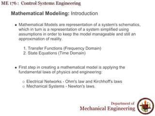
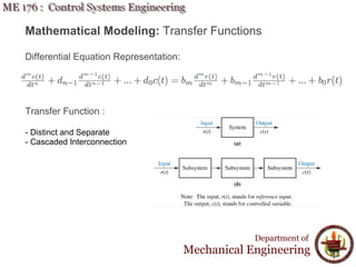
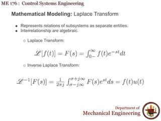
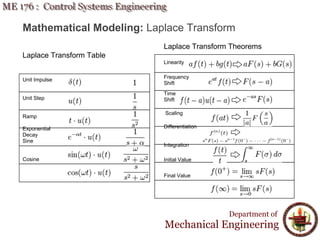
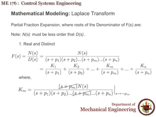
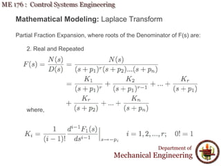
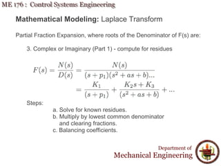
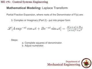
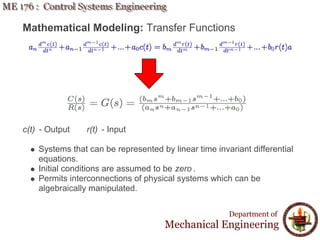
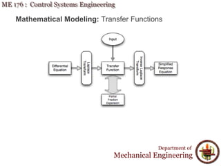
ME 176
Control Systems Engineering
Department of
Mechanical Engineering
Mathematical Modeling
Mathematical Modeling: Introduction
Mathematical Models are representation of a system's schematics,
which in turn is a representation of a system simplified using
assumptions in order to keep the model manageable and still an
approximation of reality.
1. Transfer Functions (Frequency Domain)
2. State Equations (Time Domain)
First step in creating a mathematical model is applying the
fundamental laws of physics and engineering:
Electrical Networks - Ohm's law and Kirchhoff's laws
Mechanical Systems - Newton's laws.
Department of
Mechanical Engineering
Mathematical Modeling: Transfer Functions
Differential Equation Representation:
Transfer Function :
- Distinct and Separate
- Cascaded Interconnection
Department of
Mechanical Engineering
Mathematical Modeling: Laplace Transform
Represents relations of subsystems as separate entities.
Interrelationship are algebraic.
Laplace Transform:
Inverse Laplace Transform:
Department of
Mechanical Engineering
Mathematical Modeling: Laplace Transform
Department of
Mechanical Engineering
Laplace Transform Table
Unit Impulse
Unit Step
Ramp
Exponential
Decay
Sine
Cosine
Laplace Transform Theorems
Linearity
Frequency
Shift
Time
Shift
Scaling
Differentiation
Integration
Initial Value
Final Value
Mathematical Modeling: Laplace Transform
Partial Fraction Expansion, where roots of the Denominator of F(s) are:
Note: N(s) must be less order that D(s) .
1. Real and Distinct
where,
Department of
Mechanical Engineering
Mathematical Modeling: Laplace Transform
Partial Fraction Expansion, where roots of the Denominator of F(s) are:
2. Real and Repeated
where,
Department of
Mechanical Engineering
Mathematical Modeling: Laplace Transform
Partial Fraction Expansion, where roots of the Denominator of F(s) are:
3. Complex or Imaginary (Part 1) - compute for residues
Steps:
a. Solve for known residues.
b. Multiply by lowest common denominator
and clearing fractions.
c. Balancing coefficients.
Department of
Mechanical Engineering
Mathematical Modeling: Laplace Transform
Partial Fraction Expansion, where roots of the Denominator of F(s) are:
3. Complex or Imaginary (Part 2) - put into proper form
Steps:
a. Complete squares of denominator.
b. Adjust numerator.
Department of
Mechanical Engineering
Mathematical Modeling: Transfer Functions
c(t) - Output r(t) - Input
Systems that can be represented by linear time invariant differential
equations.
Initial conditions are assumed to be zero .
Permits interconnections of physical systems which can be
algebraically manipulated.
Department of
Mechanical Engineering
Mathematical Modeling: Transfer Functions
Department of
Mechanical Engineering

Lecture 2 ME 176 2 Mathematical Modeling

  • 1.
    ME 176 Control SystemsEngineering Department of Mechanical Engineering Mathematical Modeling
  • 2.
    Mathematical Modeling: Introduction MathematicalModels are representation of a system's schematics, which in turn is a representation of a system simplified using assumptions in order to keep the model manageable and still an approximation of reality. 1. Transfer Functions (Frequency Domain) 2. State Equations (Time Domain) First step in creating a mathematical model is applying the fundamental laws of physics and engineering: Electrical Networks - Ohm's law and Kirchhoff's laws Mechanical Systems - Newton's laws. Department of Mechanical Engineering
  • 3.
    Mathematical Modeling: TransferFunctions Differential Equation Representation: Transfer Function : - Distinct and Separate - Cascaded Interconnection Department of Mechanical Engineering
  • 4.
    Mathematical Modeling: LaplaceTransform Represents relations of subsystems as separate entities. Interrelationship are algebraic. Laplace Transform: Inverse Laplace Transform: Department of Mechanical Engineering
  • 5.
    Mathematical Modeling: LaplaceTransform Department of Mechanical Engineering Laplace Transform Table Unit Impulse Unit Step Ramp Exponential Decay Sine Cosine Laplace Transform Theorems Linearity Frequency Shift Time Shift Scaling Differentiation Integration Initial Value Final Value
  • 6.
    Mathematical Modeling: LaplaceTransform Partial Fraction Expansion, where roots of the Denominator of F(s) are: Note: N(s) must be less order that D(s) . 1. Real and Distinct where, Department of Mechanical Engineering
  • 7.
    Mathematical Modeling: LaplaceTransform Partial Fraction Expansion, where roots of the Denominator of F(s) are: 2. Real and Repeated where, Department of Mechanical Engineering
  • 8.
    Mathematical Modeling: LaplaceTransform Partial Fraction Expansion, where roots of the Denominator of F(s) are: 3. Complex or Imaginary (Part 1) - compute for residues Steps: a. Solve for known residues. b. Multiply by lowest common denominator and clearing fractions. c. Balancing coefficients. Department of Mechanical Engineering
  • 9.
    Mathematical Modeling: LaplaceTransform Partial Fraction Expansion, where roots of the Denominator of F(s) are: 3. Complex or Imaginary (Part 2) - put into proper form Steps: a. Complete squares of denominator. b. Adjust numerator. Department of Mechanical Engineering
  • 10.
    Mathematical Modeling: TransferFunctions c(t) - Output r(t) - Input Systems that can be represented by linear time invariant differential equations. Initial conditions are assumed to be zero . Permits interconnections of physical systems which can be algebraically manipulated. Department of Mechanical Engineering
  • 11.
    Mathematical Modeling: TransferFunctions Department of Mechanical Engineering