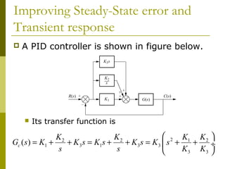
Downloaded 452 times

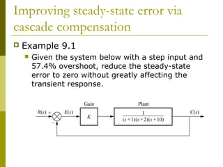
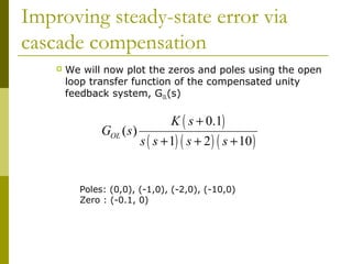
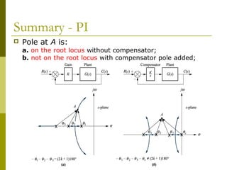
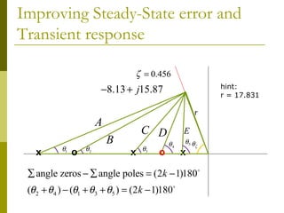
![Improving steady-state error via
cascade compensation
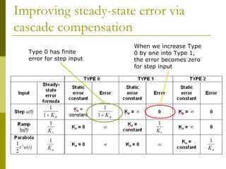
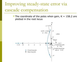
Example for PI controller:
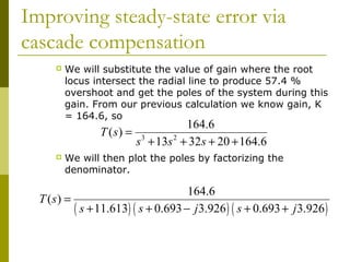
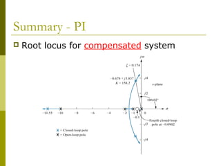
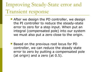
Figure below is an example of a unity feedback
system with gain, K. Point A is on the root
locus which means the [sum of zeros angle] –
[sum of poles angle] = odd multiples of 180̊.](https://image.slidesharecdn.com/controlchap8-131231194115-phpapp02/85/Control-chap8-16-320.jpg)
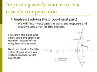

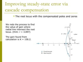
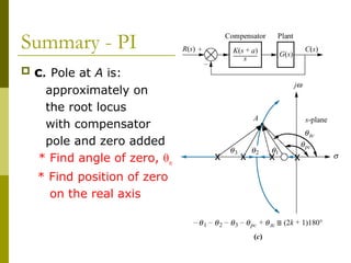
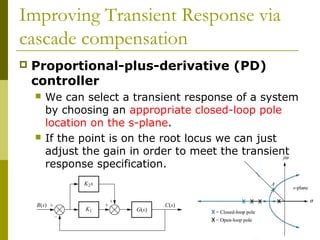
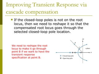
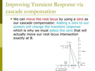
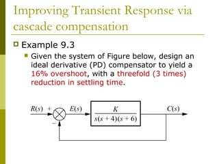
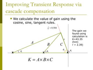
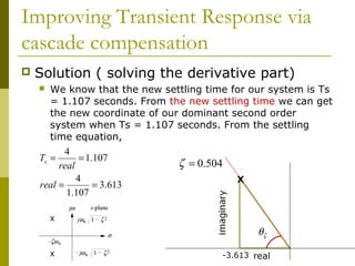
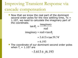
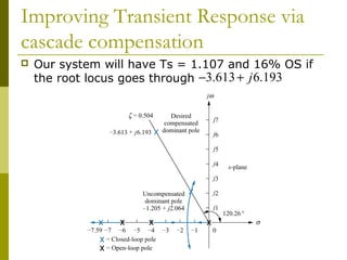
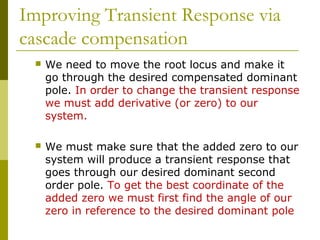
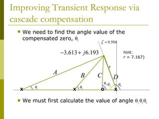
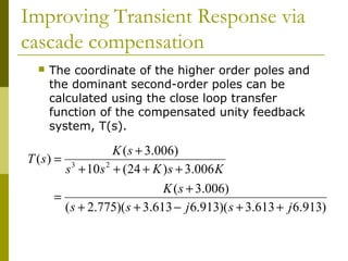
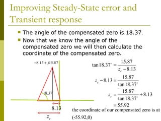
![Improving Transient Response via
cascade compensation
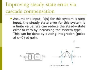
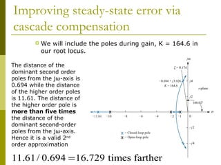
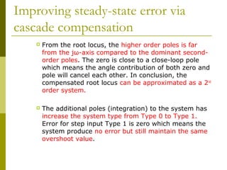
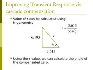
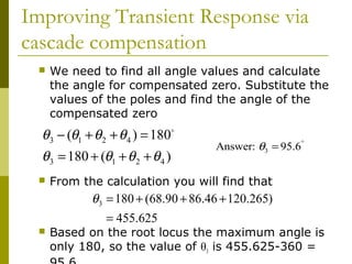
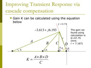
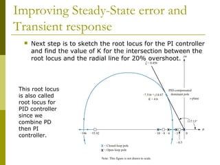
The value of the compensated zero angle can be calculated
using the fact that the [summation of zeros angle] minus
[summation of poles angle]=odd multiple of 180̊. We must use
the sine, cosine and tangent rules to calculate the angles.
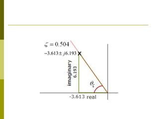
ζ = 0.504
−3.613 + j 6.193
A
X
θ1
B
X
θ2
hint:
r = 7.167)
r
C
θ3 θ
ζ
O
D
θ4
X
∑ angle zeros − ∑ angle poles = 180o](https://image.slidesharecdn.com/controlchap8-131231194115-phpapp02/85/Control-chap8-62-320.jpg)
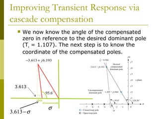
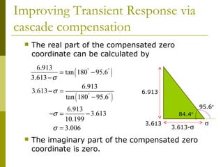
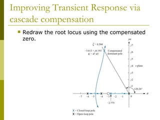

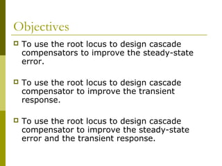
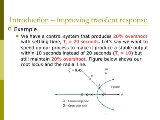
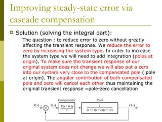
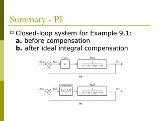
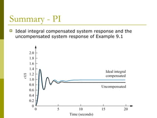
This document discusses using cascade compensation to improve control system performance. Cascade compensation involves adding additional poles and zeros to the open-loop transfer function. This can improve the transient response by placing poles farther out in the s-plane, and improve steady-state error by increasing the system type. An example shows designing a PI controller to reduce steady-state error to zero without affecting the 57.4% overshoot transient response. Pole-zero cancellation is used to maintain the original transient response while increasing the system type.