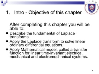
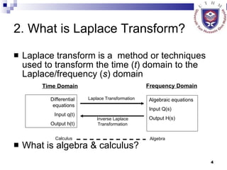
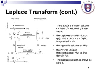
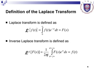
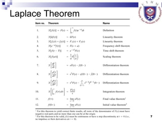
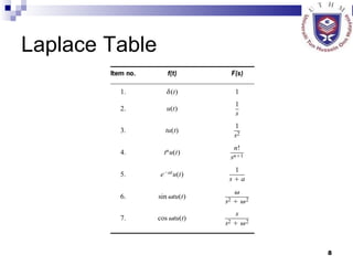
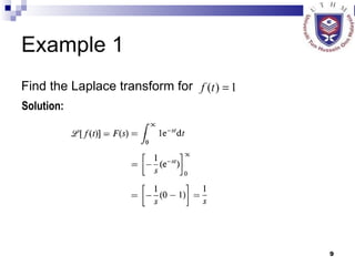
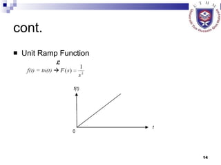
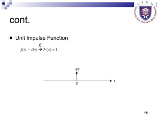
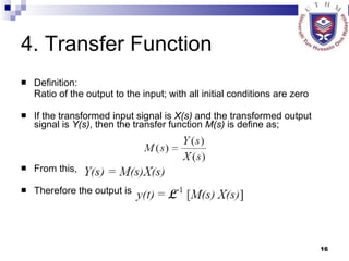
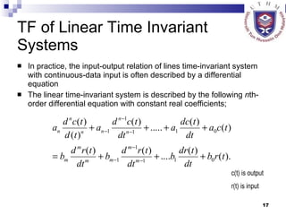
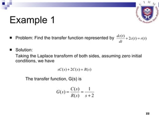
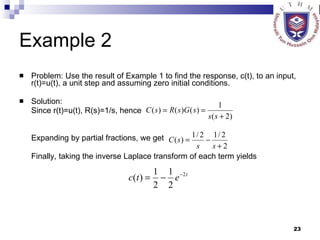
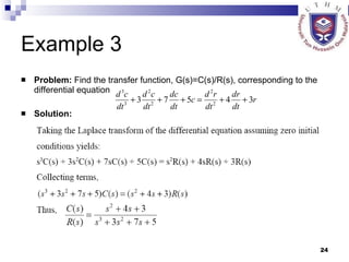
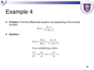
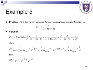
This document provides an overview of analog control systems and Laplace transforms. It introduces key concepts like Laplace transforms, common time domain inputs, transfer functions, and modeling electrical, mechanical and electromechanical systems using block diagrams and mathematical models. Examples are provided to illustrate Laplace transforms, transfer functions, and analyzing system response using poles, zeros and stability analysis.

1. Chapter 2 Analog Control System Eddy Irwan Shah Bin Saadon Dept. of Electrical Engineering PPD, UTHM [email_address] 019-7017679

2. Outline: Introduction Laplace Transform – Table/ Theorem/ Eg. Common Time Domain Input Function Transfer Function – Open/ Closed Loop & Eg. Electrical Elements Modelling – Table & Eg. Mechanical Elements Modelling - Table & Eg. Block Diagram Reduction - Table & Eg. System Response – Poles/ Zeros, Second Order, Steady State Error, Stability Analysis

3. Intro - Objective of this chapter After completing this chapter you will be able to: Describe the fundamental of Laplace transforms. Apply the Laplace transform to solve linear ordinary differential equations. Apply Mathematical model, called a transfer function for linear time-invariant electrical, mechanical and electromechanical systems.

4. 2. What is Laplace Transform? Laplace transform is a method or techniques used to transform the time ( t ) domain to the Laplace/frequency ( s ) domain What is algebra & calculus? Time Domain Frequency Domain Differential equations Input q(t) Output h(t) Algebraic equations Input Q(s) Output H(s) Calculus Algebra Laplace Transformation Inverse Laplace Transformation

5. Laplace Transform (cont.) The Laplace transform solution consists of the following three steps: the Laplace transformation of q1(t) and (r dhldt + h = Gq) to frequency domain the algebraic solution for H(s) the inverse Laplace transformation of H(s) to time domain h(t). The calculus solution is shown as step 4.

6. Definition of the Laplace Transform Laplace transform is defined as Inverse Laplace transform is defined as L L -1

7. Laplace Theorem

8. Laplace Table

9. Example 1 Find the Laplace transform for Solution:

10. Example 2 Find the Laplace transform for Solution:

11. Example 3 Find the inverse Laplace transform of Solution: Expanding F(s) by partial fraction: Where, Then, taking the inverse Laplace transform

12. Example 4 Given the ,solve for y ( t ) if all initial conditions are zero. Use the Laplace transform method . Solution: Substitute the corresponding F ( s ) for each term: Solving for the response: Where, K 1 = 1 when s=0 K 2 =-2 when s=-4 K 3 = 1 when s=-8 Hence

13. 3. Common Time Domain Input Functions Unit Step Function

14. Unit Ramp Function cont.

15. Unit Impulse Function cont.

16. 4. Transfer Function Definition: Ratio of the output to the input; with all initial conditions are zero If the transformed input signal is X(s) and the transformed output signal is Y(s) , then the transfer function M(s) is define as; From this, Therefore the output is

17. TF of Linear Time Invariant Systems In practice, the input-output relation of lines time-invariant system with continuous-data input is often described by a differential equation The linear time-invariant system is described by the following n th-order differential equation with constant real coefficients; c(t) is output r(t) is input

18. cont. Taking the Laplace transform of both sides, If we assume that all initial conditions are zero, hence Now, form the ratio of output transform, C(s) divided by input transform. The ratio, G(s) is called transfer function.

19. cont. The transfer function can be represented as a block diagram General block diagram

20. Block Diagram of Open Loop System

21. Block Diagram of Closed Loop System

22. Example 1 Problem: Find the transfer function represented by Solution: Taking the Laplace transform of both sides, assuming zero initial conditions, we have The transfer function, G(s) is

23. Example 2 Problem: Use the result of Example 1 to find the response, c(t), to an input, r(t)=u(t), a unit step and assuming zero initial conditions. Solution: Since r(t)=u(t), R(s)=1/s, hence Expanding by partial fractions, we get Finally, taking the inverse Laplace transform of each term yields

24. Example 3 Problem: Find the transfer function, G(s)=C(s)/R(s), corresponding to the differential equation Solution:

25. Example 4 Problem: Find the differential equation corresponding to the transfer function, Solution:

26. Example 5 Problem: Find the ramp response for a system whose transfer function is, Solution: