Download as PDF, PPTX
![Curve Fitting using inbuilt functions
polyfit(x,y,n)
finds the coefficients of a polynomial P(x) of degree n that fits
the data
It uses least-square minimization
n = 1 (linear fit)
[P] = polyfit(X,Y,N)
returns P, a matrix containing the slope and the x intercept for a
linear fit
[Y] = polyval(P,X)
calculates the Y values for every X point on the line of best fit
Dr. Summiya Parveen 27](https://image.slidesharecdn.com/dataapproximationinmathematicalmodellingregressionanalysisandcurvefitting-180714044958/75/Data-Approximation-in-Mathematical-Modelling-Regression-Analysis-and-Curve-Fitting-27-2048.jpg)
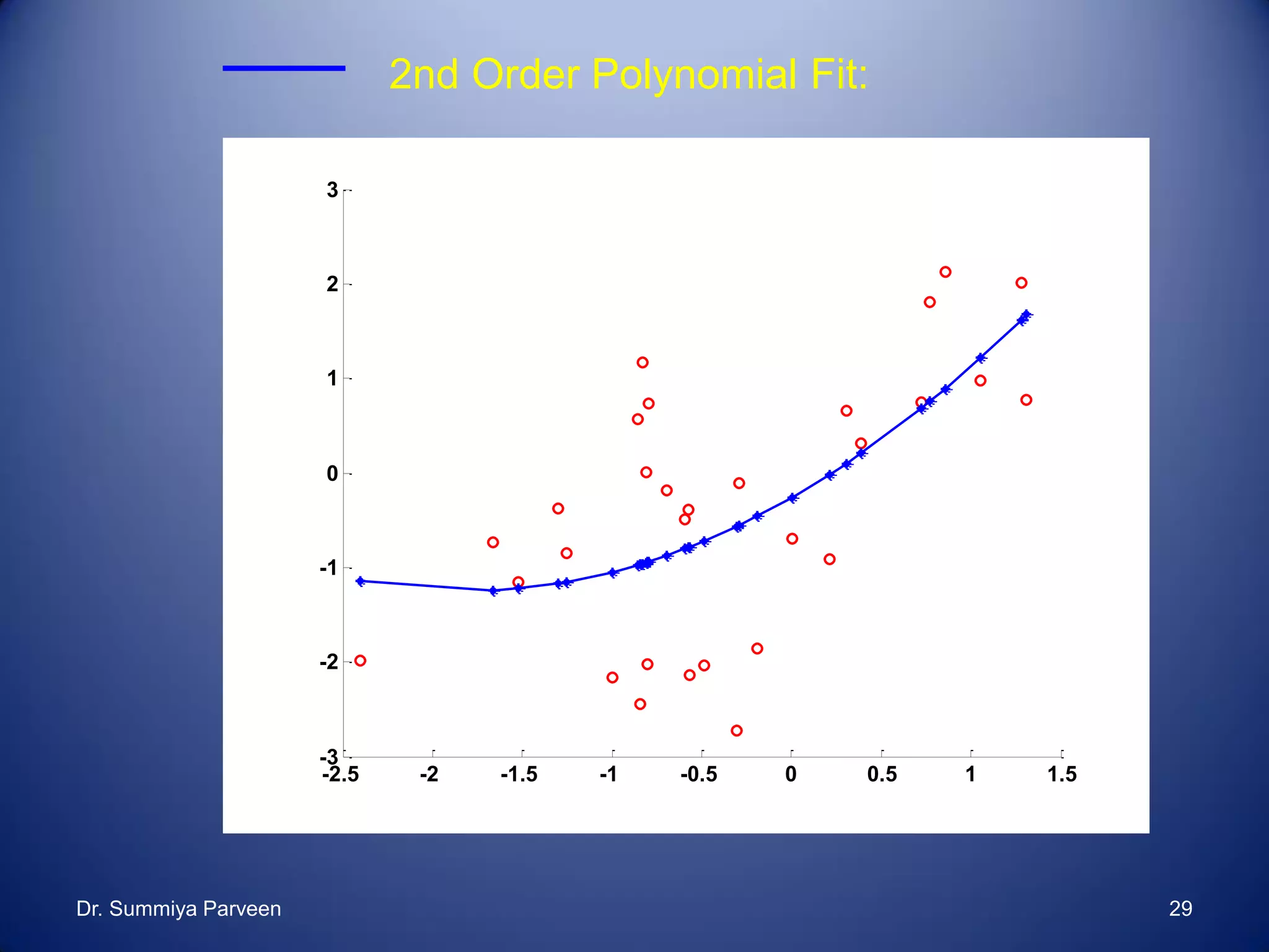
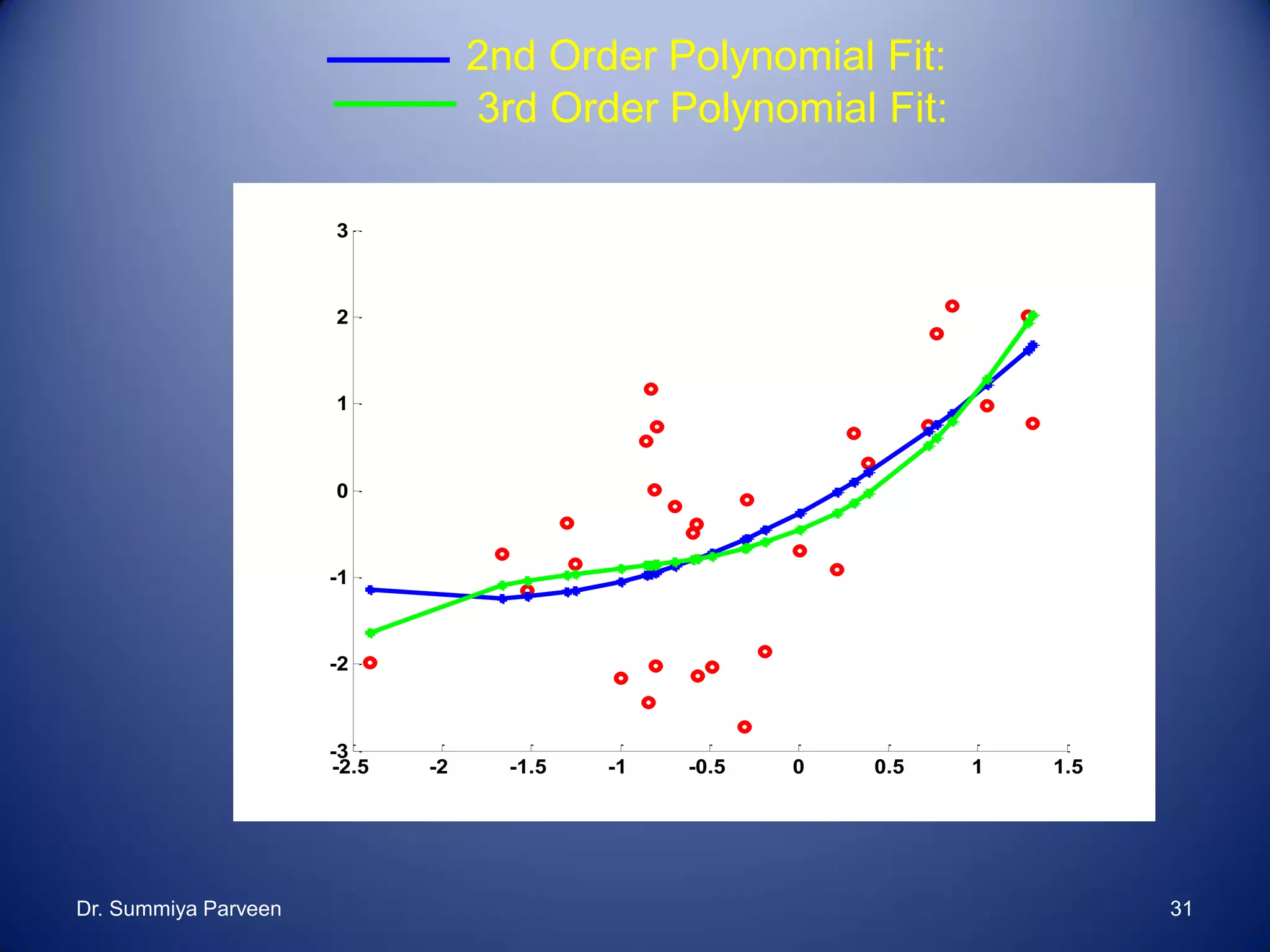
![Curve Fitting Example
• 2nd Order Polynomial Fit:
%read data
[var1, var2] = textread(‘week8_testdata2.txt','%f%f','headerlines',1)
% Calculate 2nd order polynomial fit
P2 = polyfit(var1,var2,2);
Y2 = polyval(P2,var1);
%Plot fit
close all
figure(1)
hold on
plot(var1,var2,'ro')
[sortedvar1, sortind] = sort(var1)
plot(sortedvar1,Y2(sortind),'b*-')Dr. Summiya Parveen 28](https://image.slidesharecdn.com/dataapproximationinmathematicalmodellingregressionanalysisandcurvefitting-180714044958/75/Data-Approximation-in-Mathematical-Modelling-Regression-Analysis-and-Curve-Fitting-28-2048.jpg)


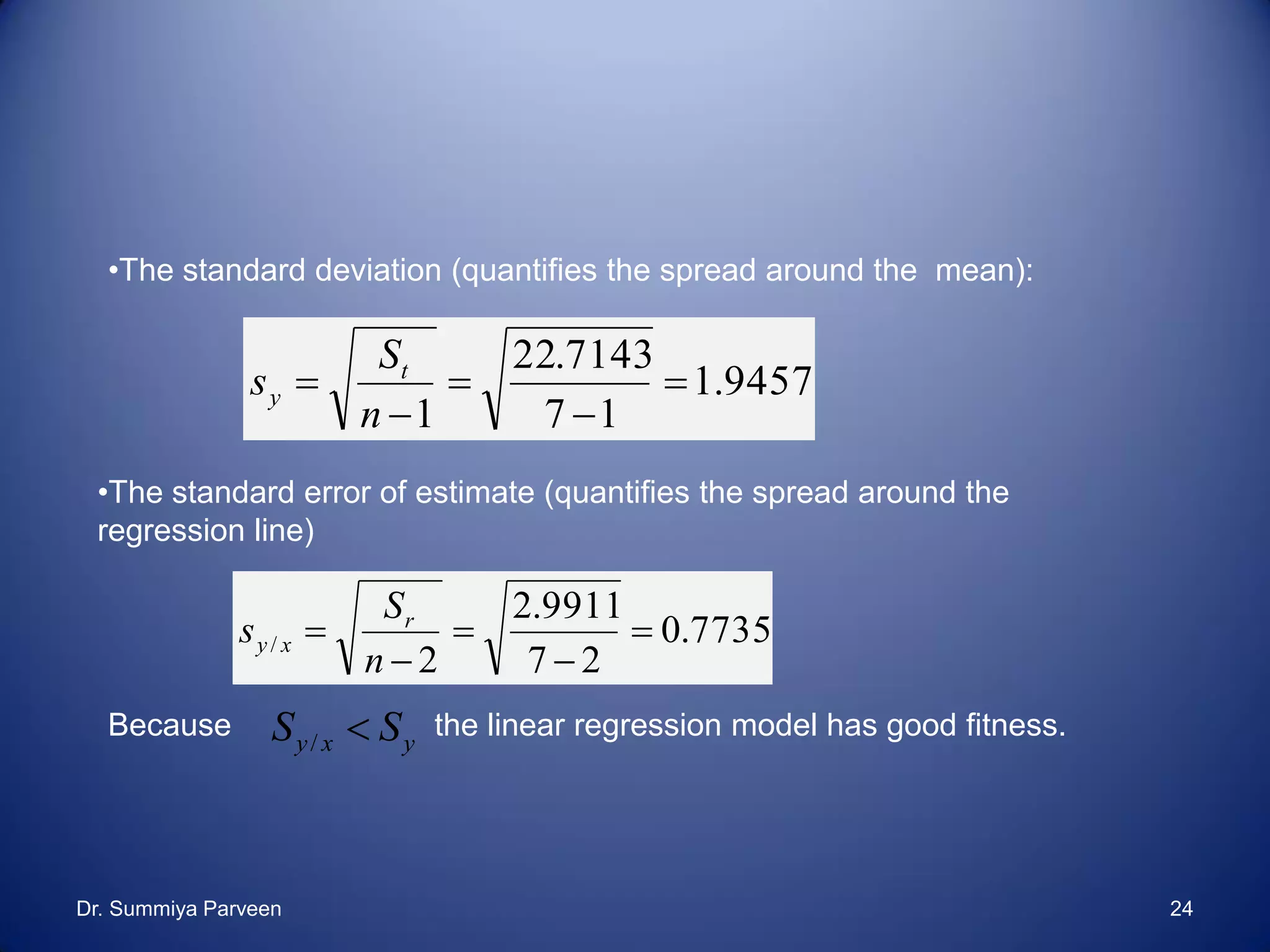
The document discusses regression analysis, a predictive modeling technique that examines the relationship between dependent and independent variables, and it covers various types of regression methods, including linear, non-linear, polynomial, and multiple linear regression. The concepts of goodness of fit, error analysis, statistical measures like the coefficient of determination, and the standard error of regression are explained with examples. Additionally, there is a focus on implementing regression in MATLAB, showcasing polynomial curve fitting using built-in functions.
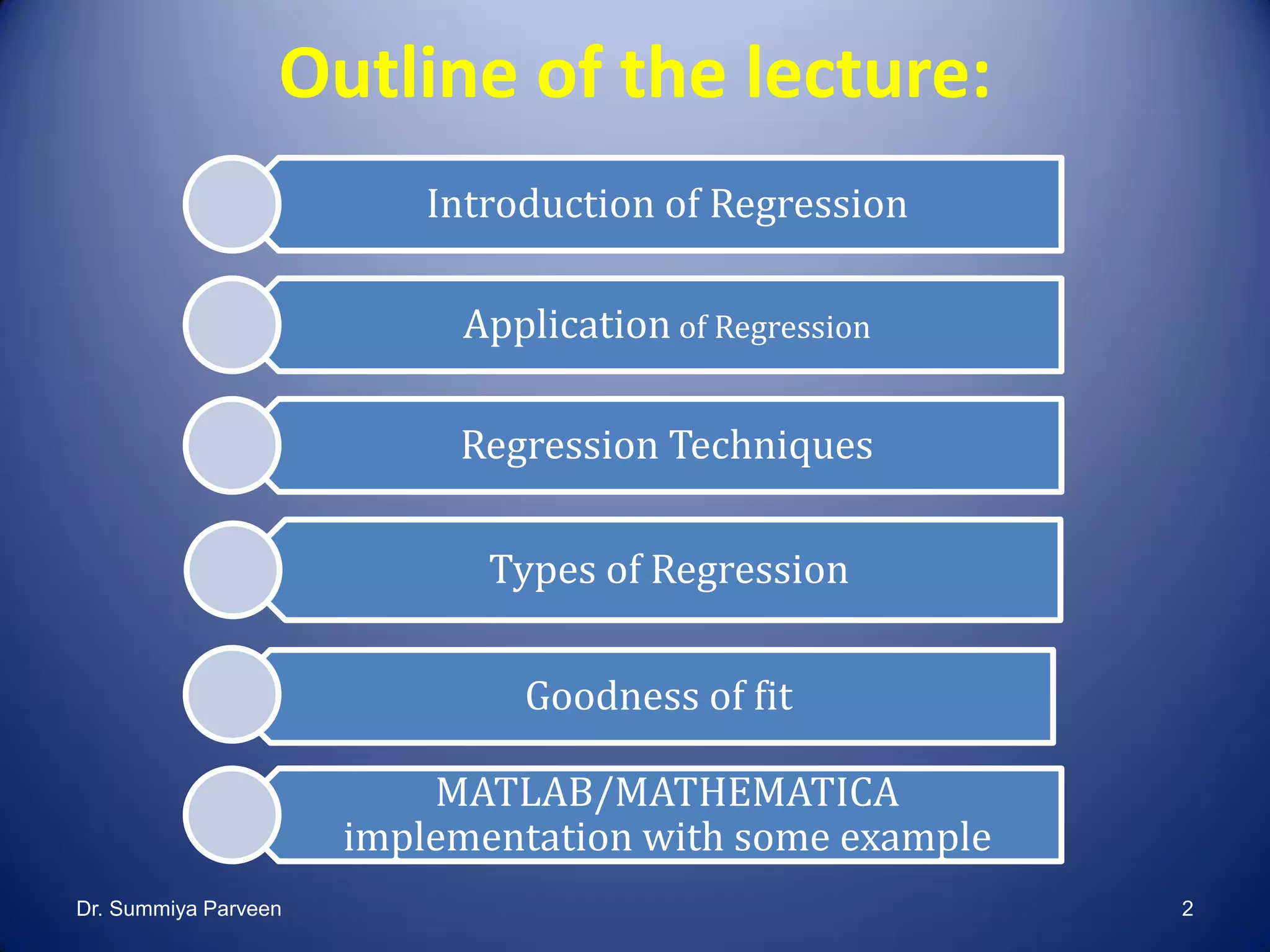
Overview of regression analysis and its importance in predictive modeling. Introduction covers outline of lecture.
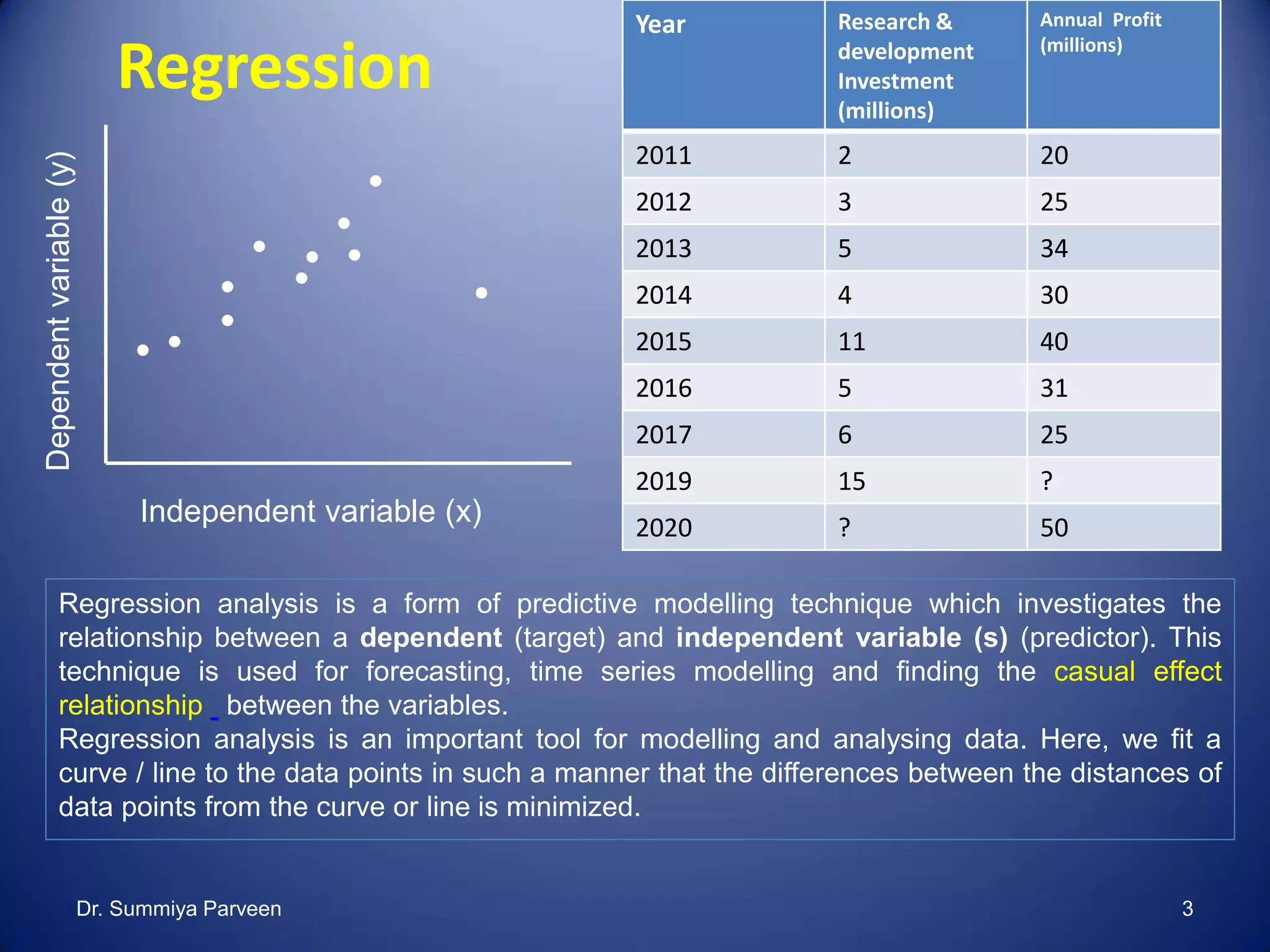
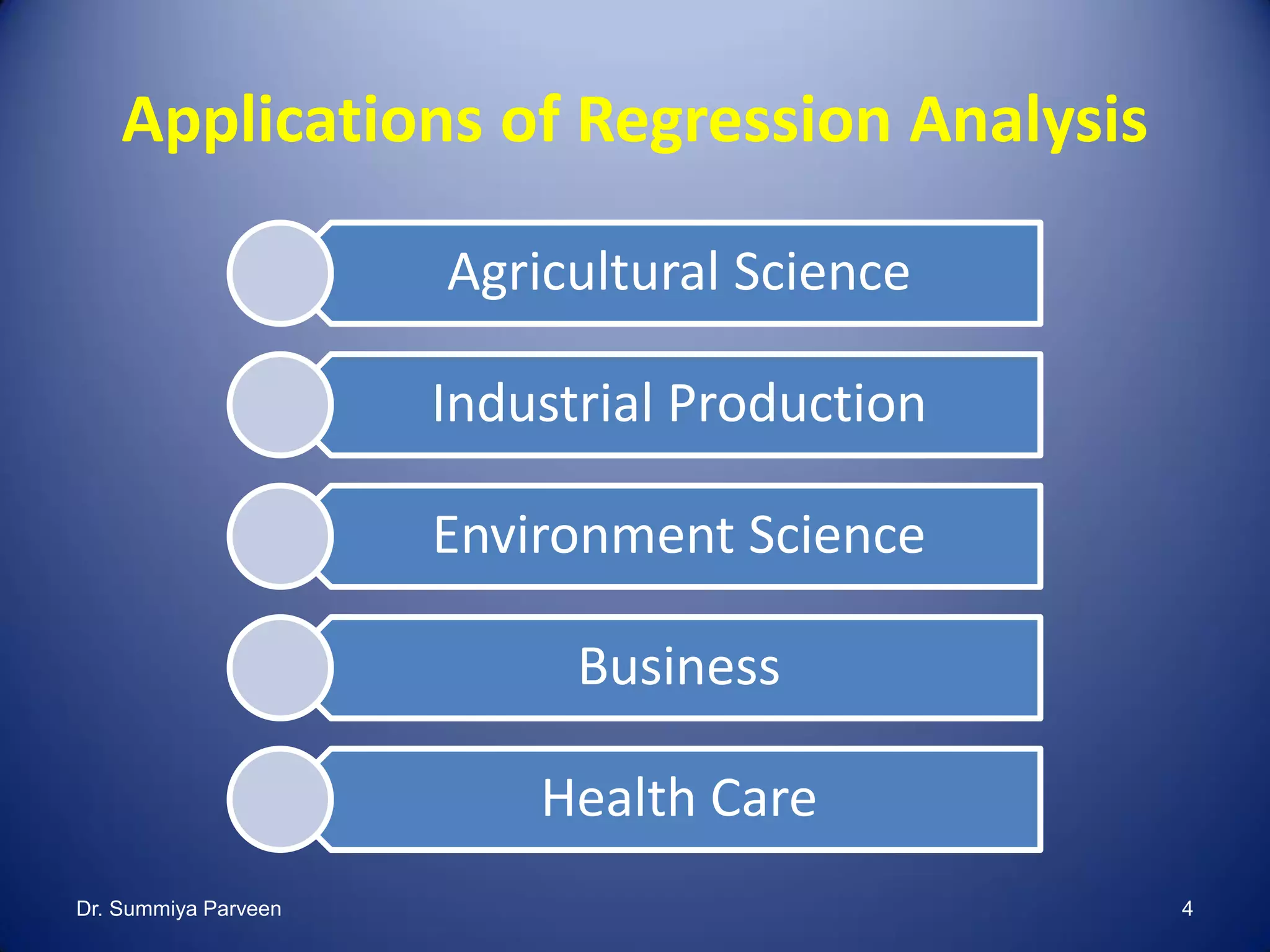
Explains the relationship between dependent and independent variables, along with real-life applications in various fields.
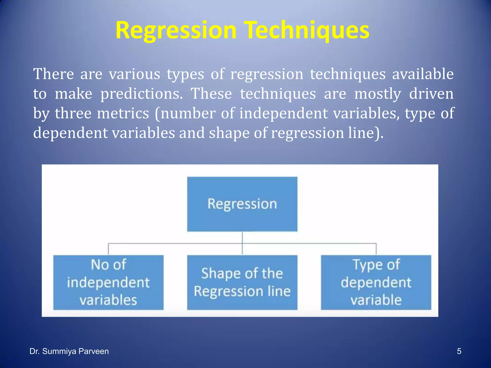
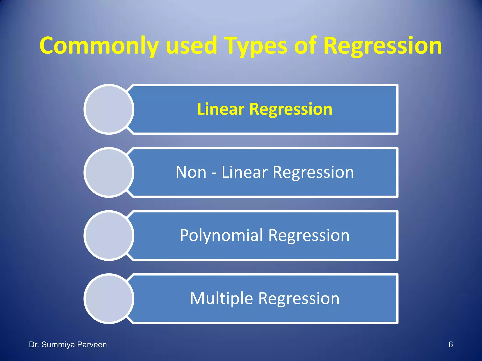
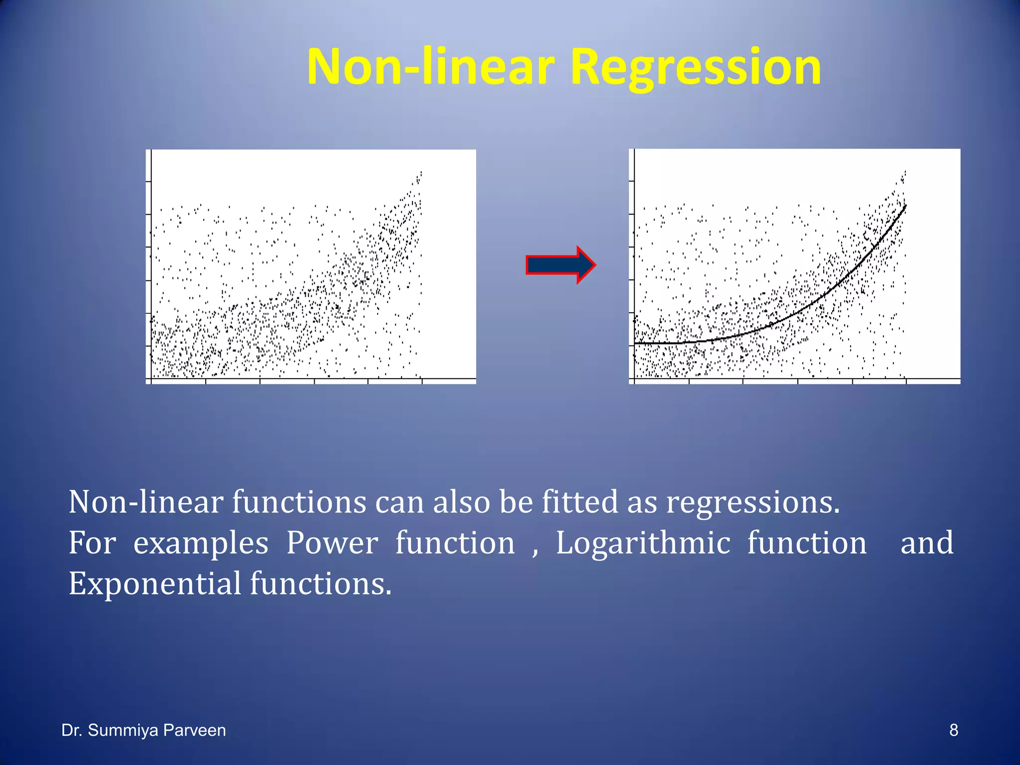
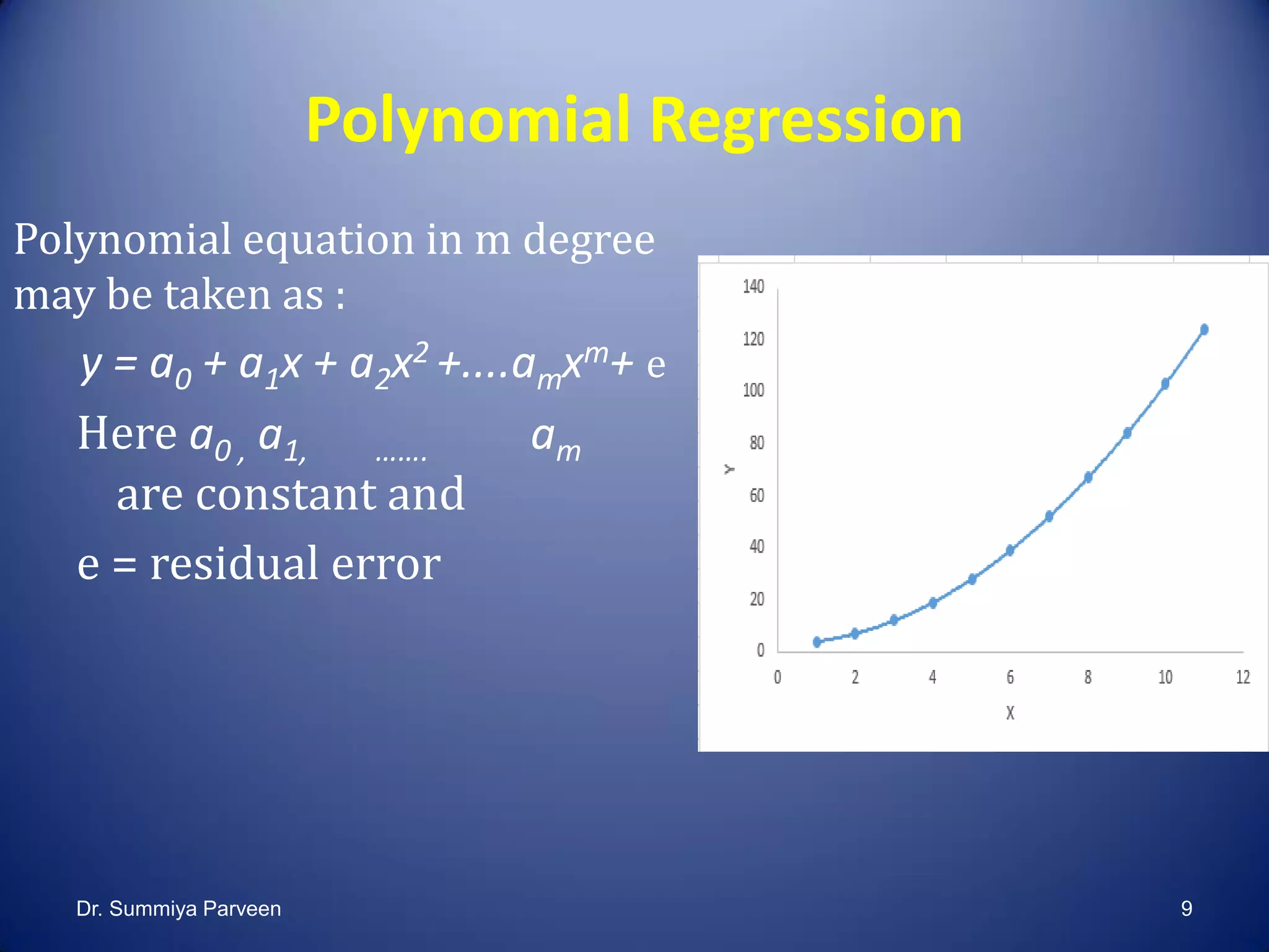
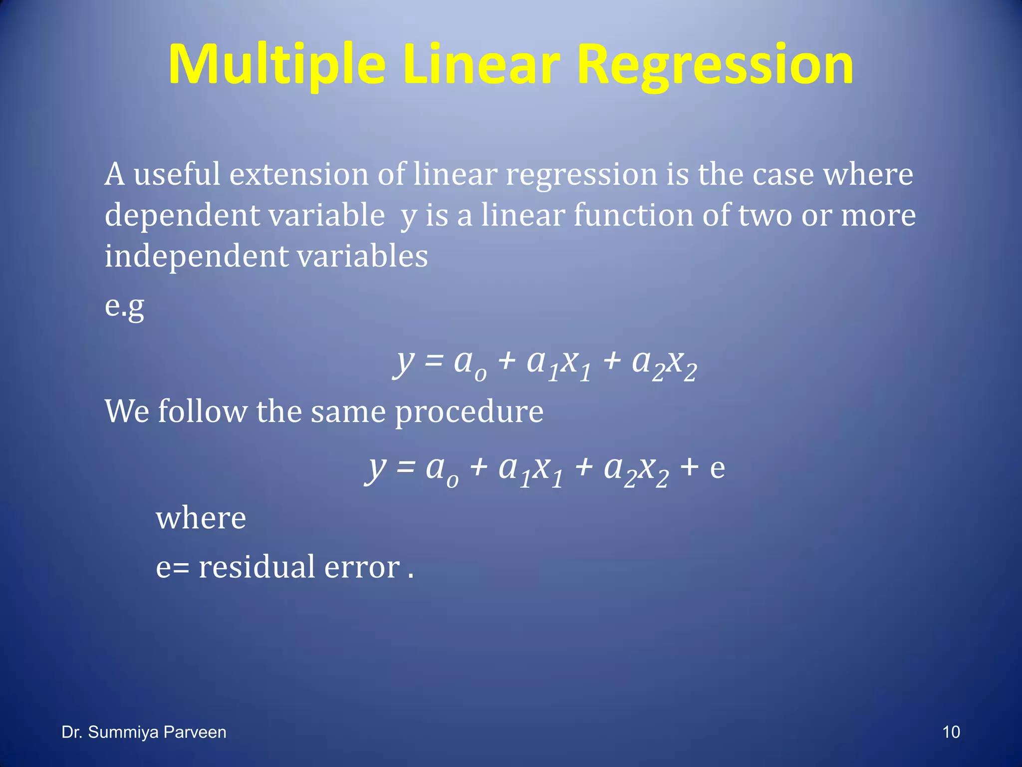
Discussion on various regression techniques including linear, non-linear, polynomial, and multiple regression.
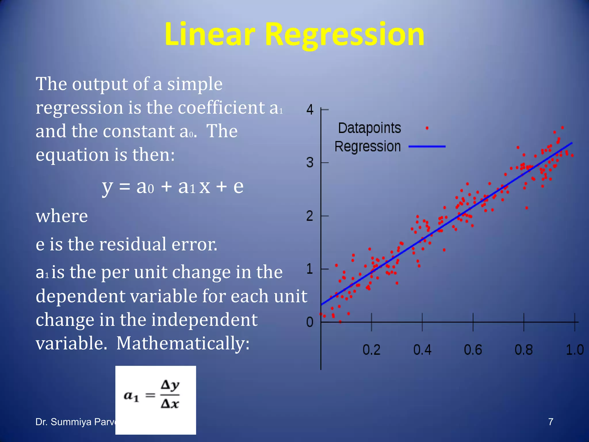
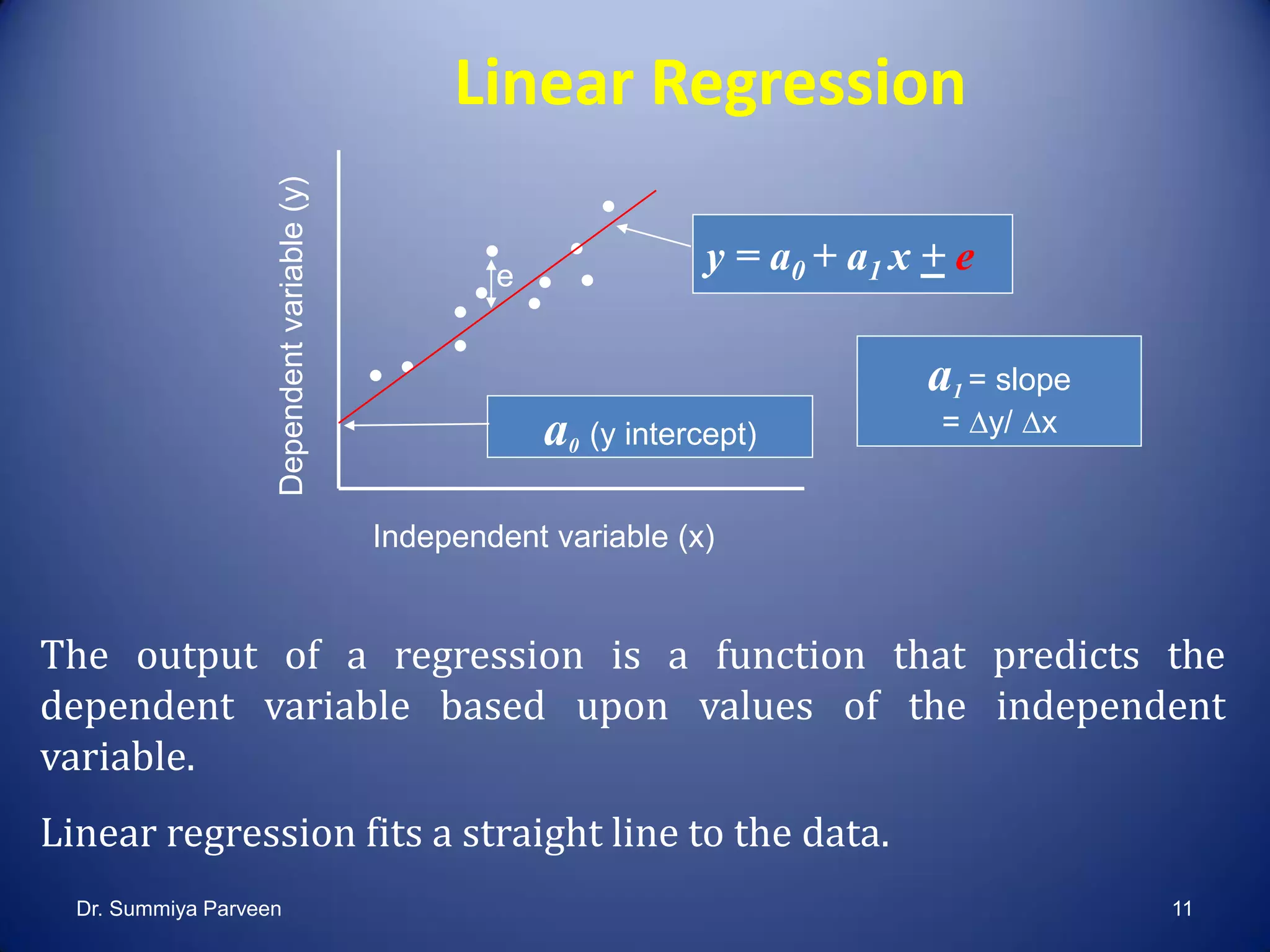
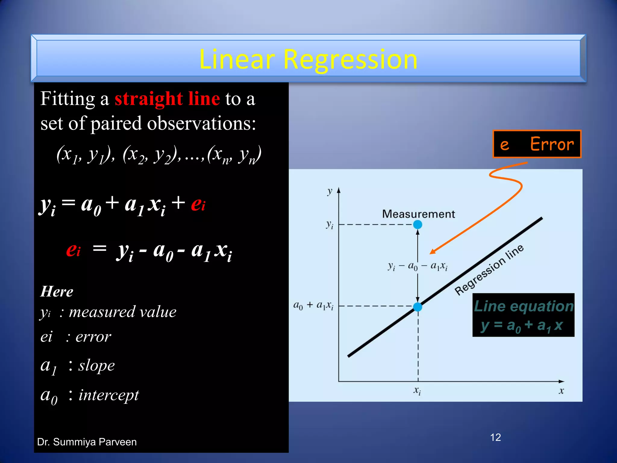
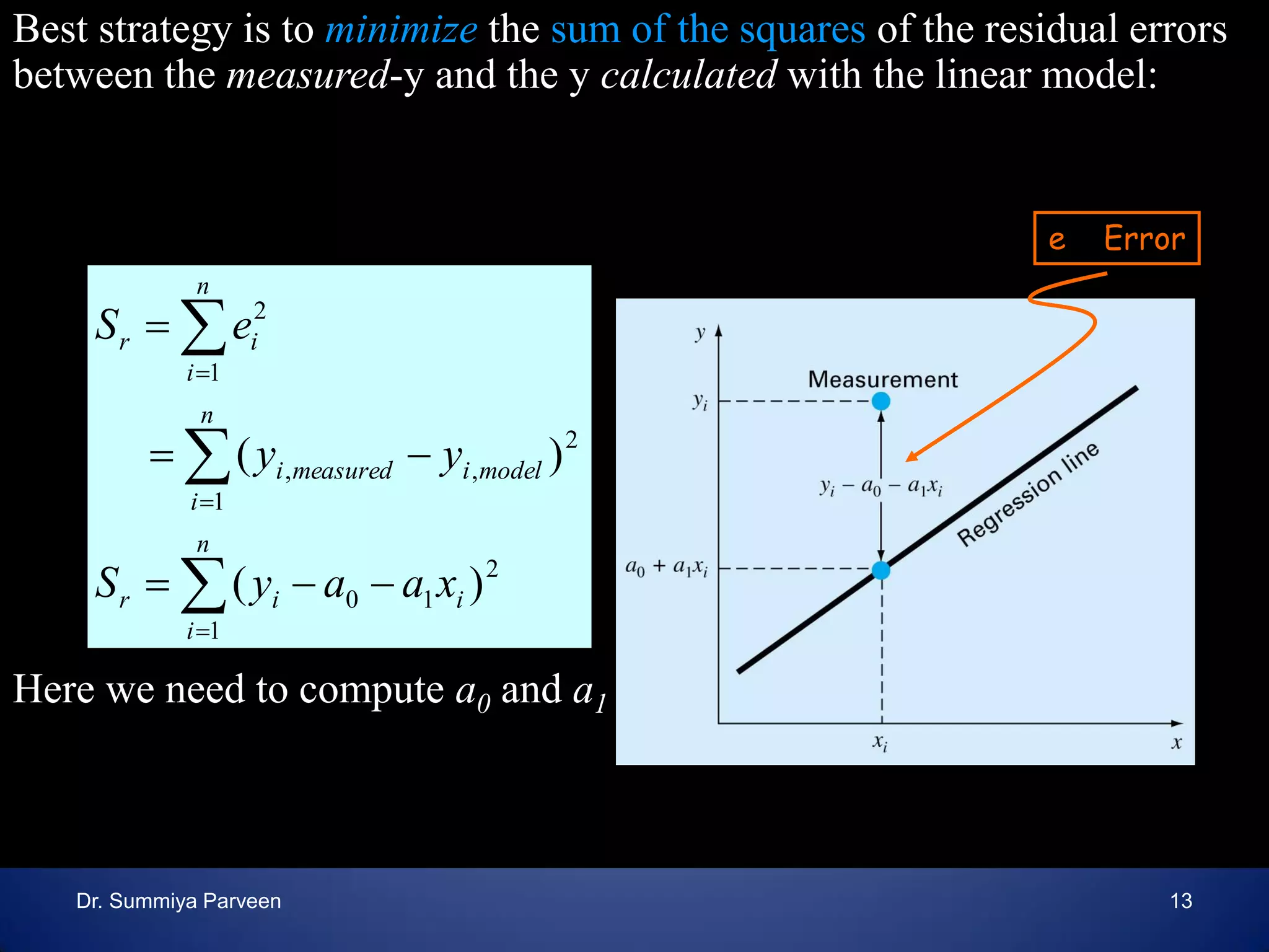
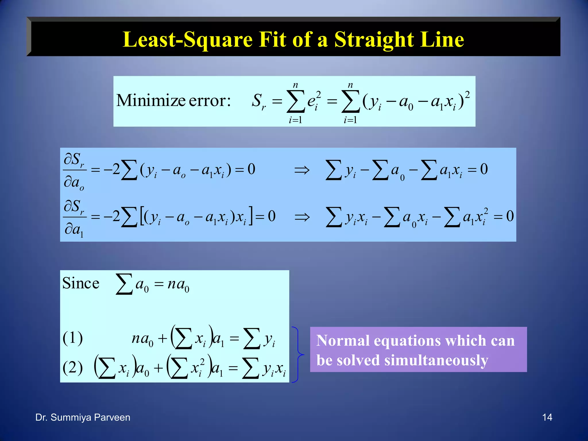
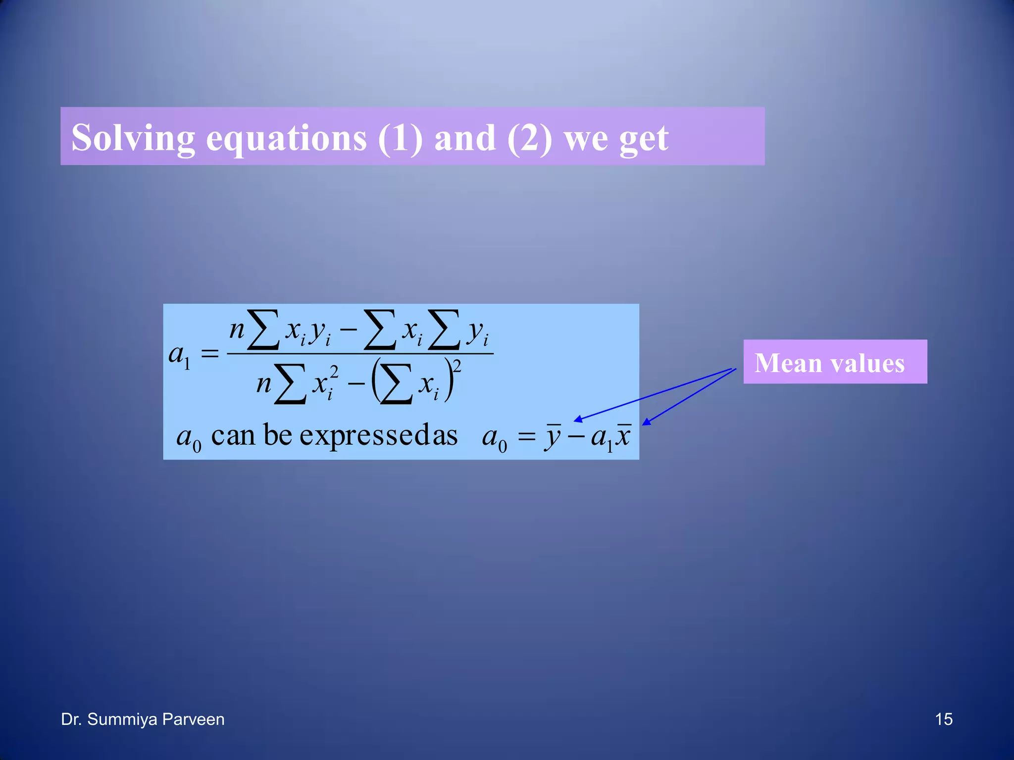
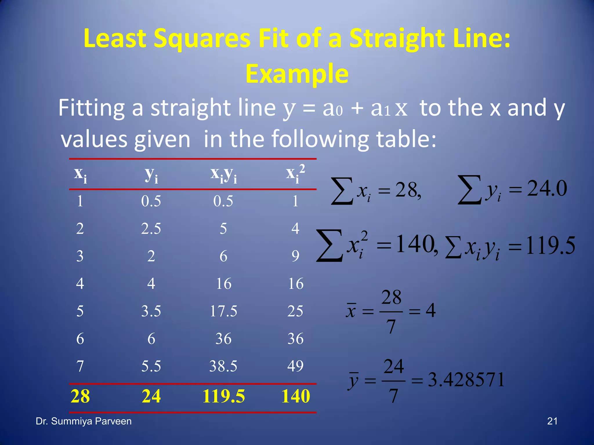
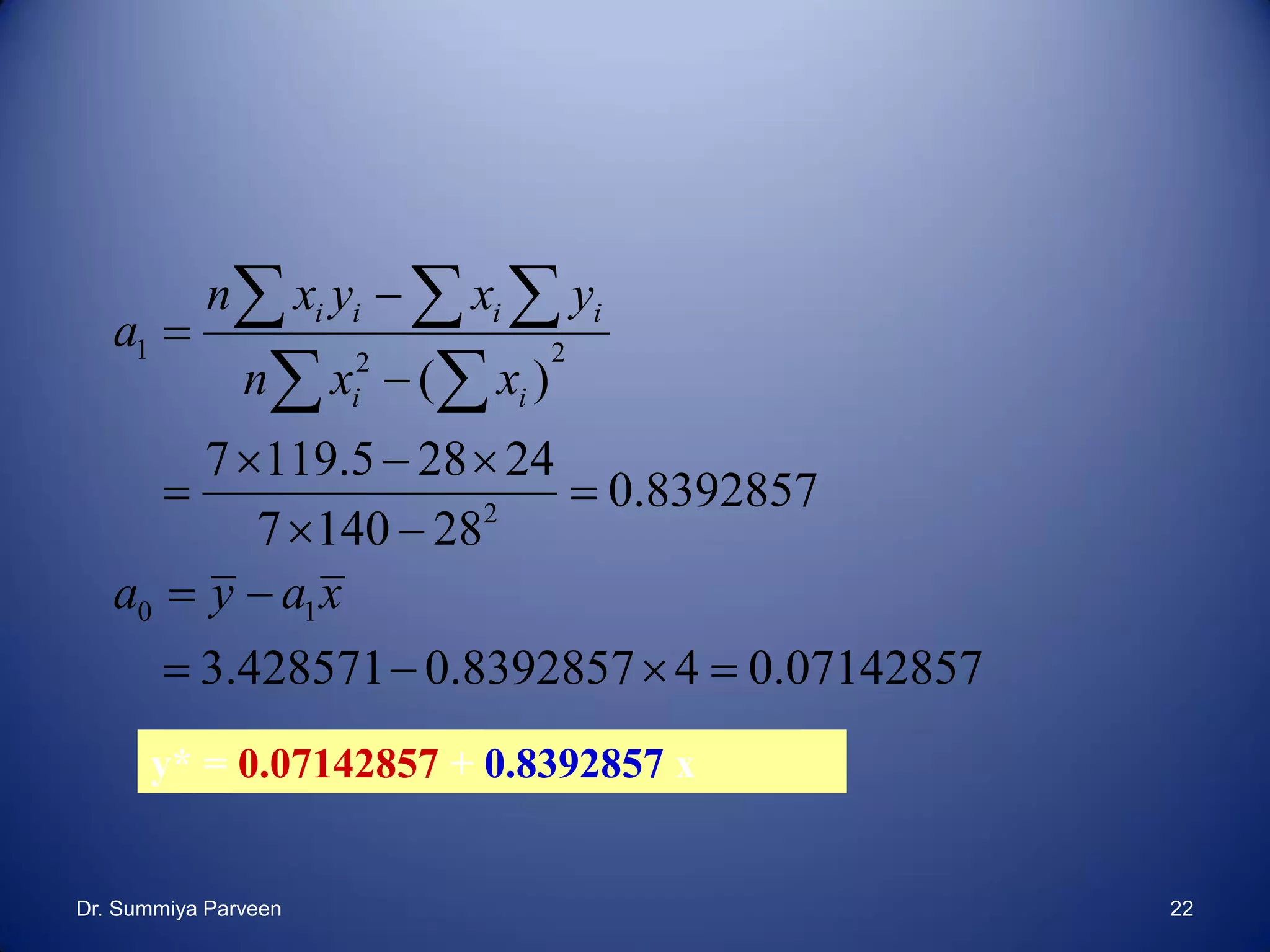
Detailed explanation of linear regression, the fitting of the line, and the least-squares method to minimize errors.
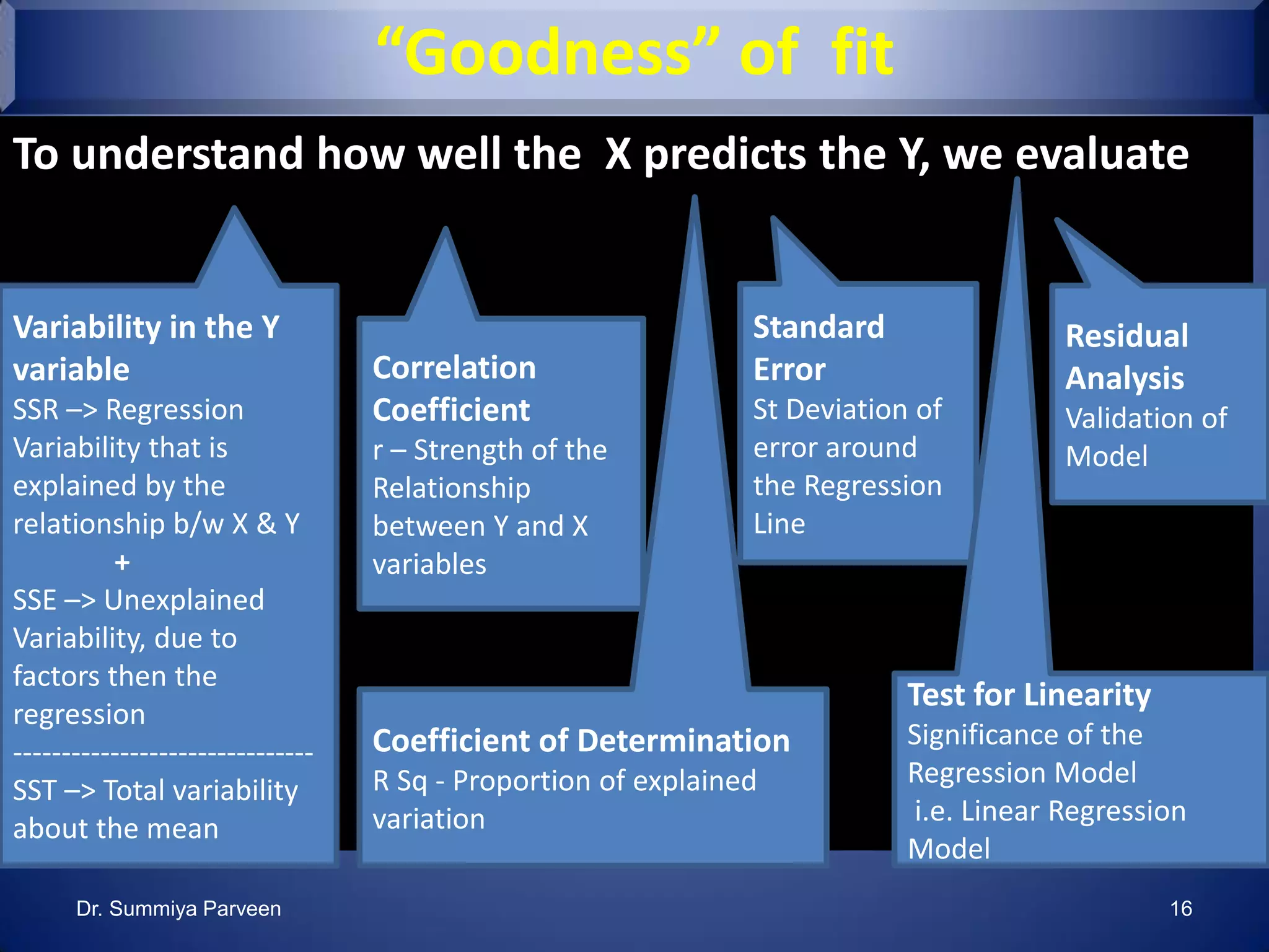
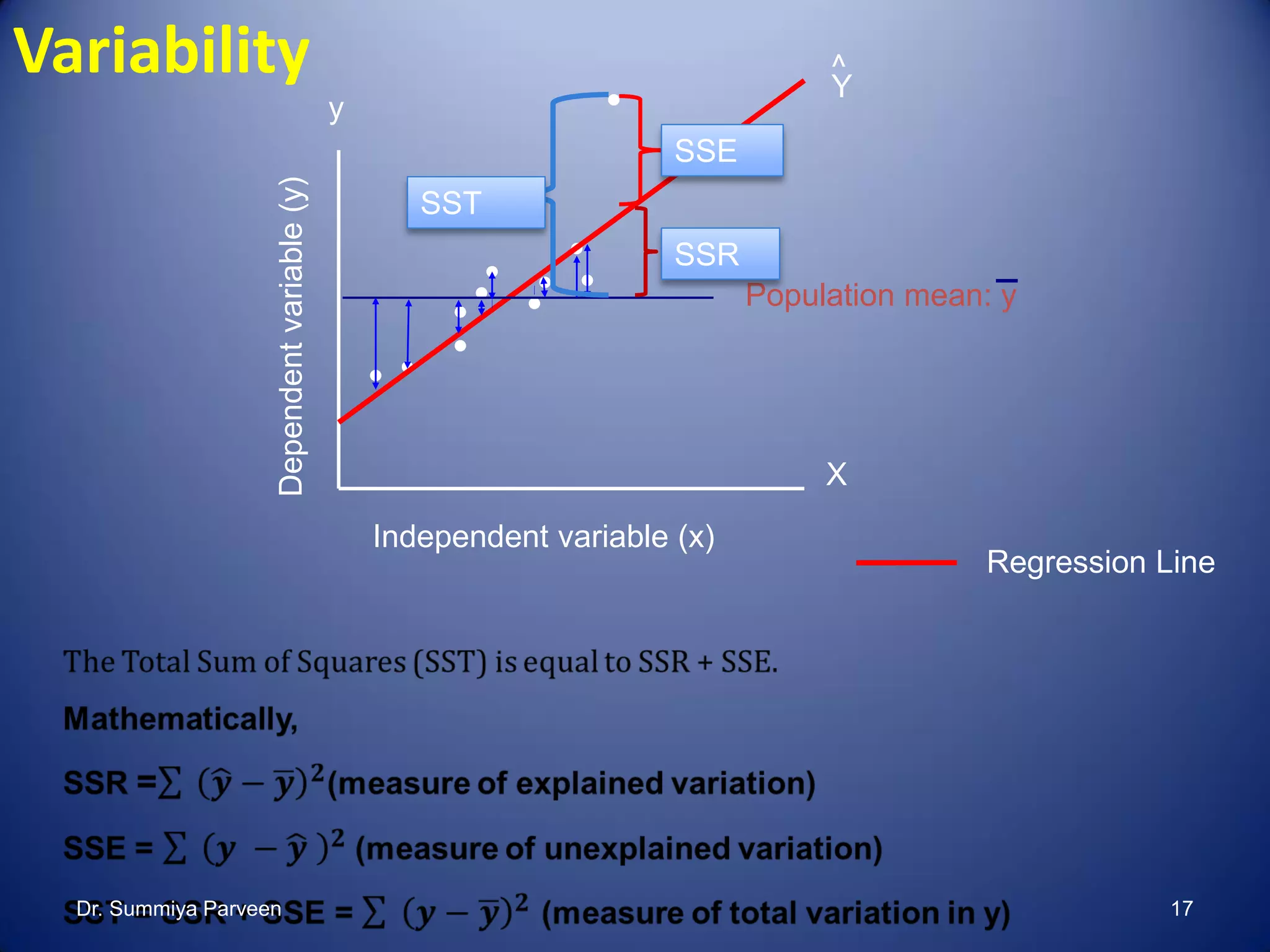
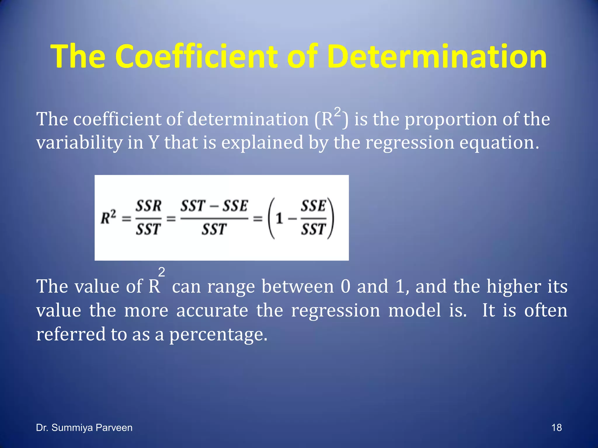
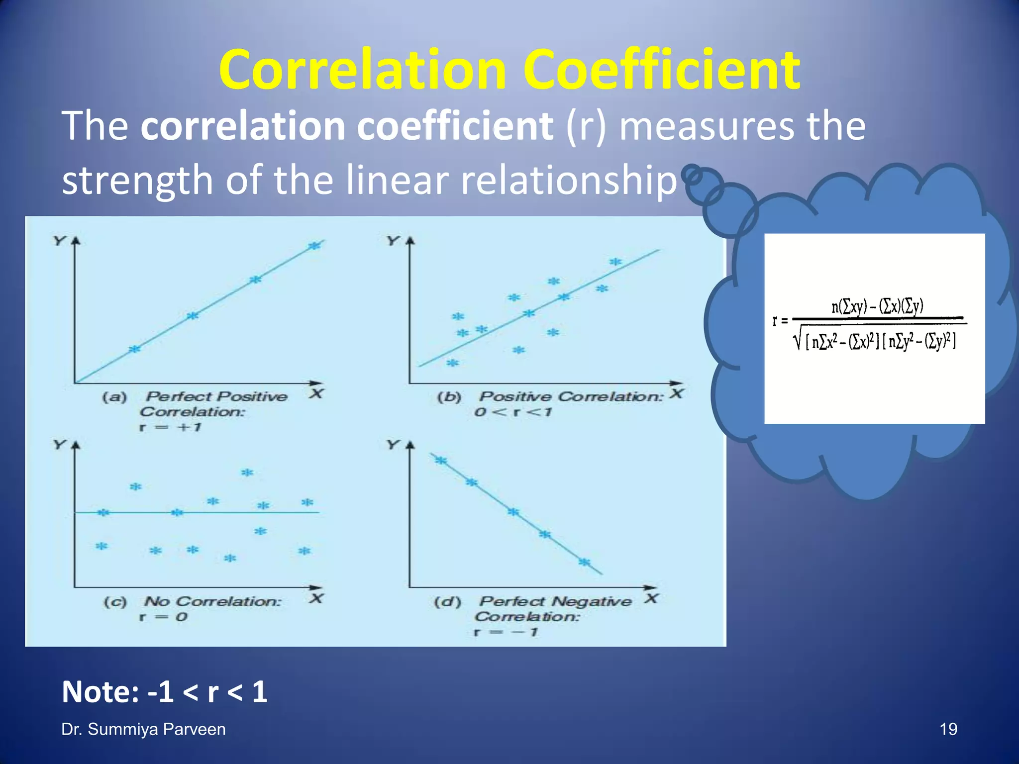
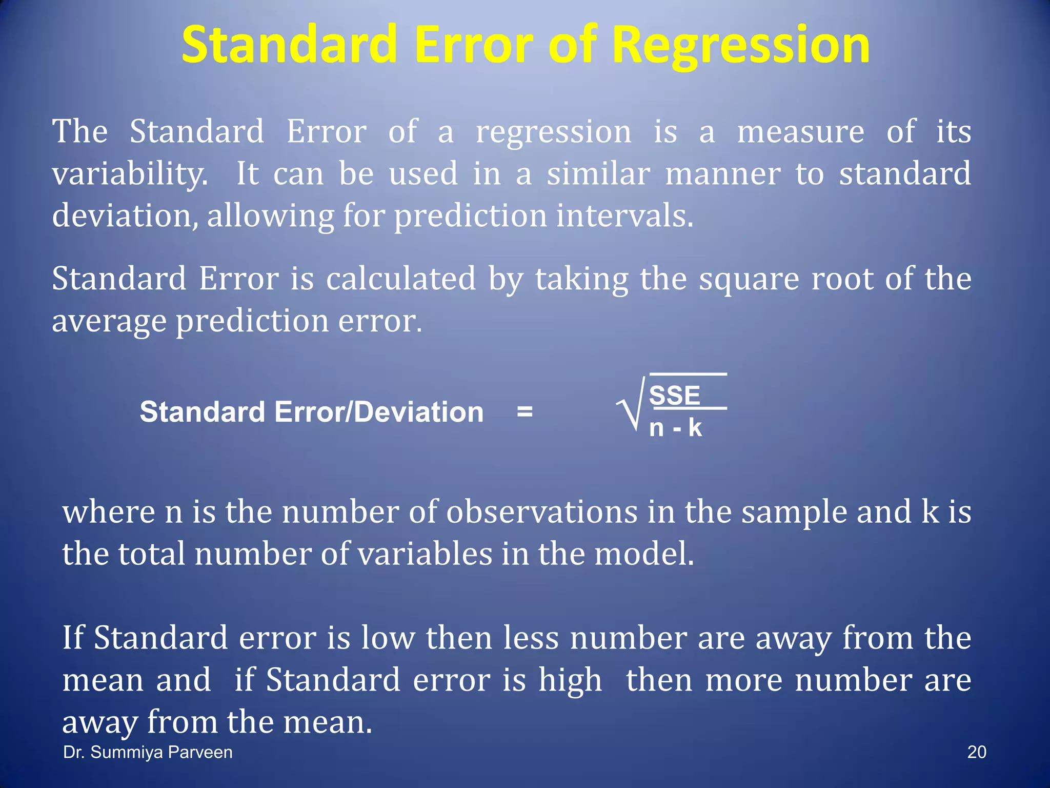
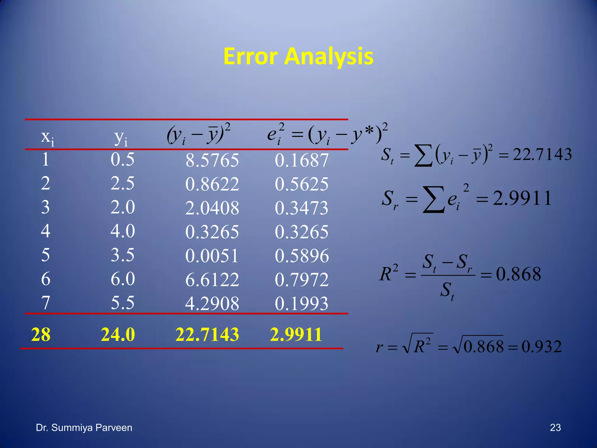
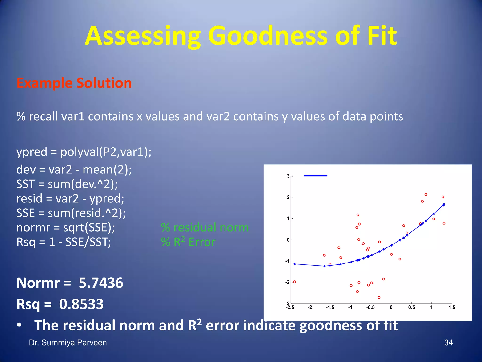
Explains model performance metrics like R-squared, standard error, correlation coefficient, and residual analysis.
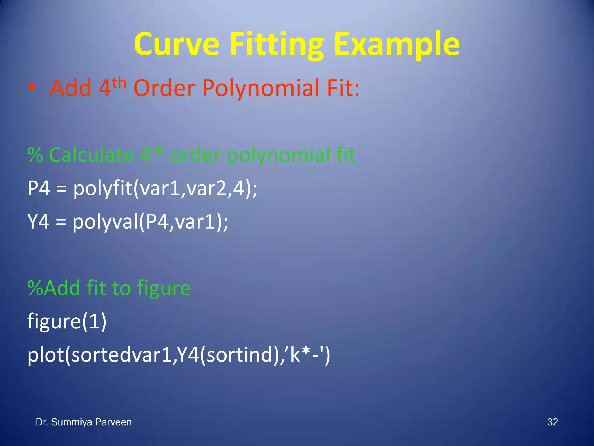
Examples on fitting data using MATLAB, including code snippets for polynomial fitting techniques.
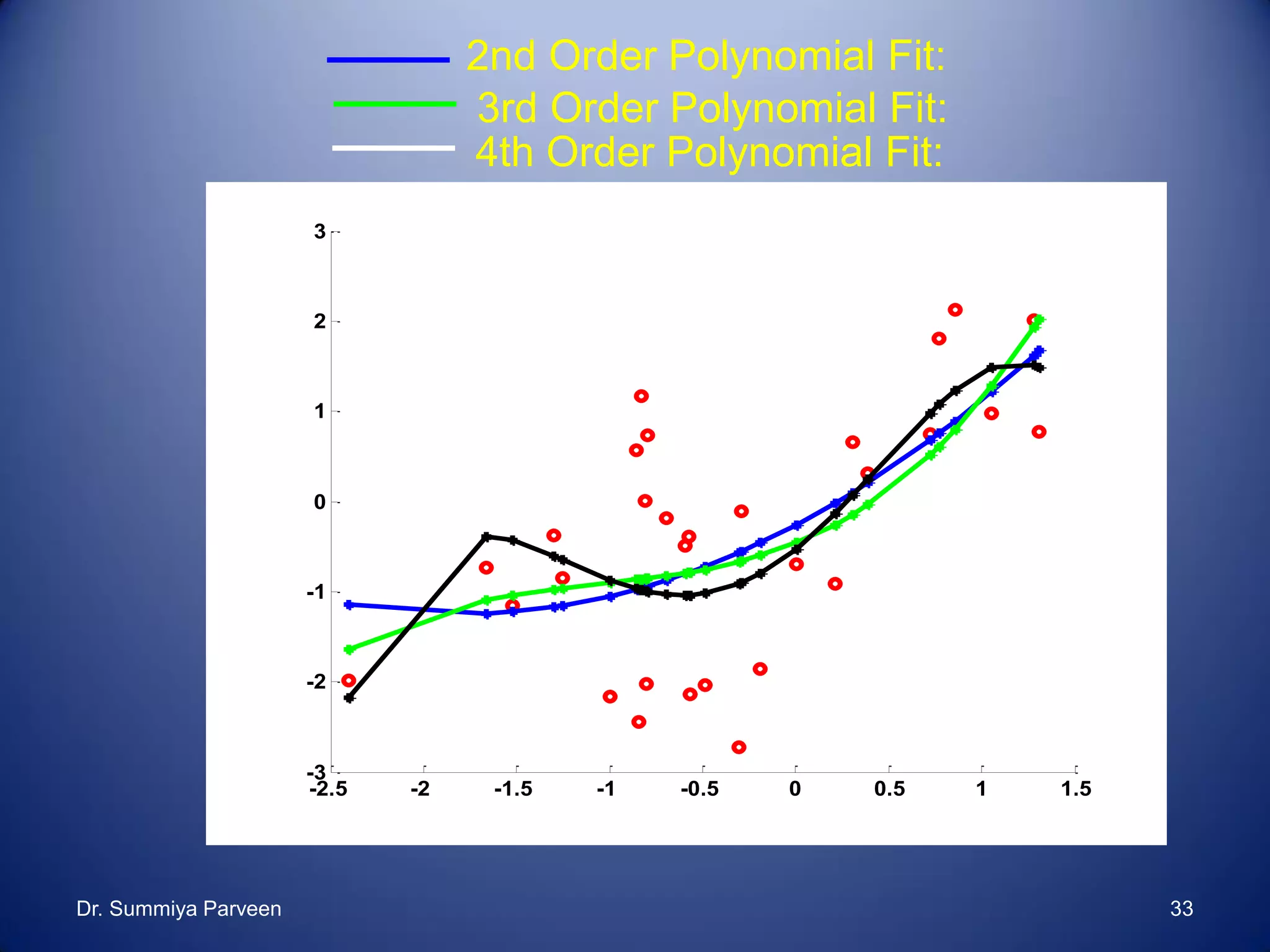
Graphical representation of polynomial fits and discusses limitations of polynomial fitting techniques.
Closing remarks and appreciation for participation.