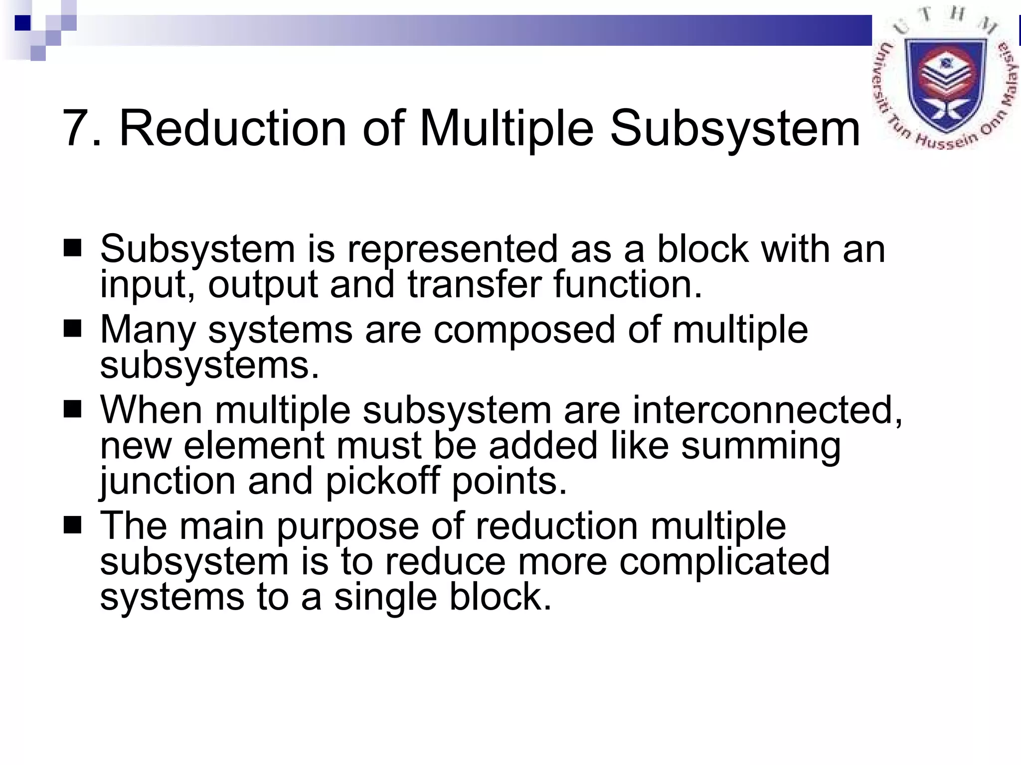
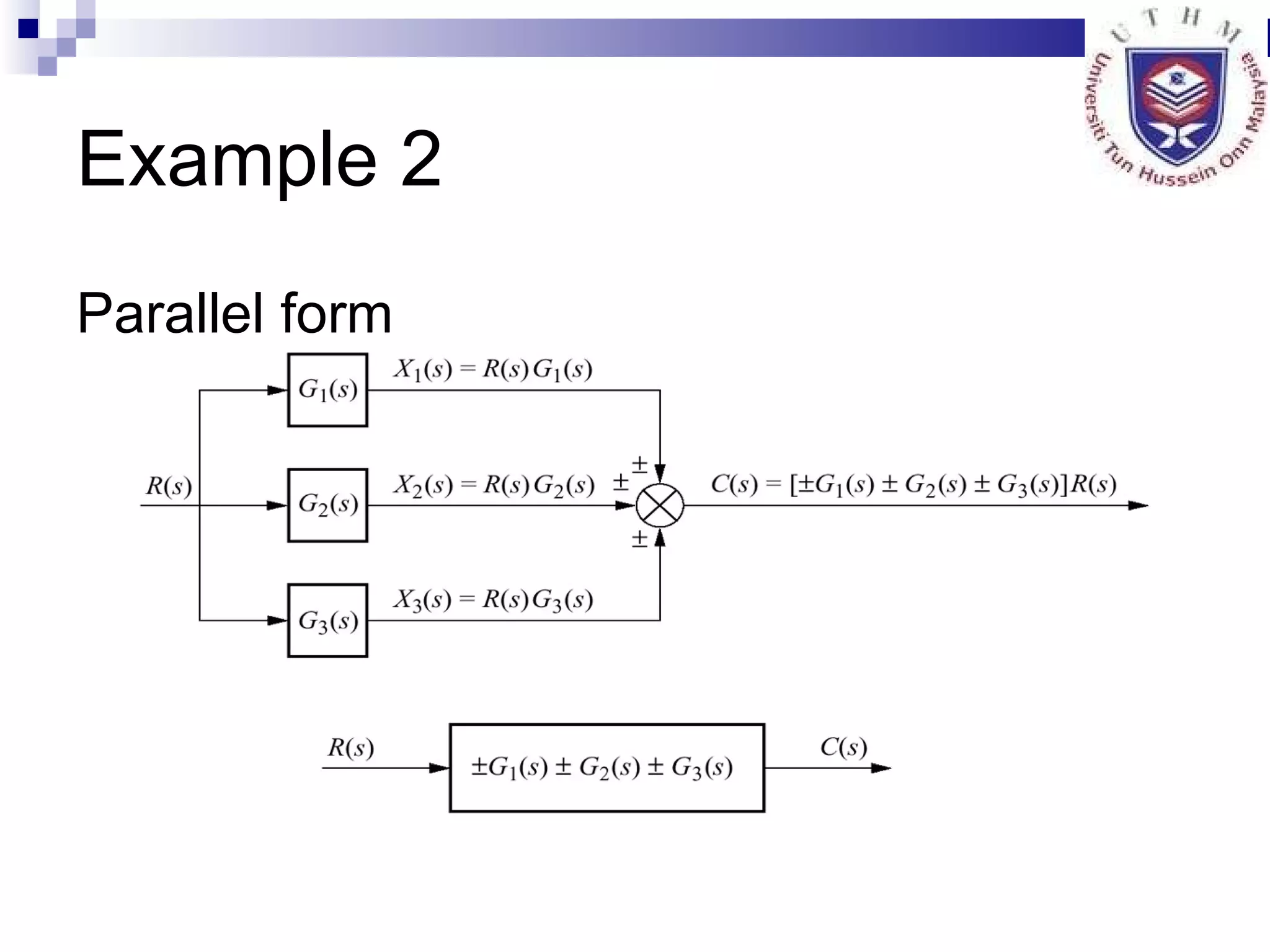
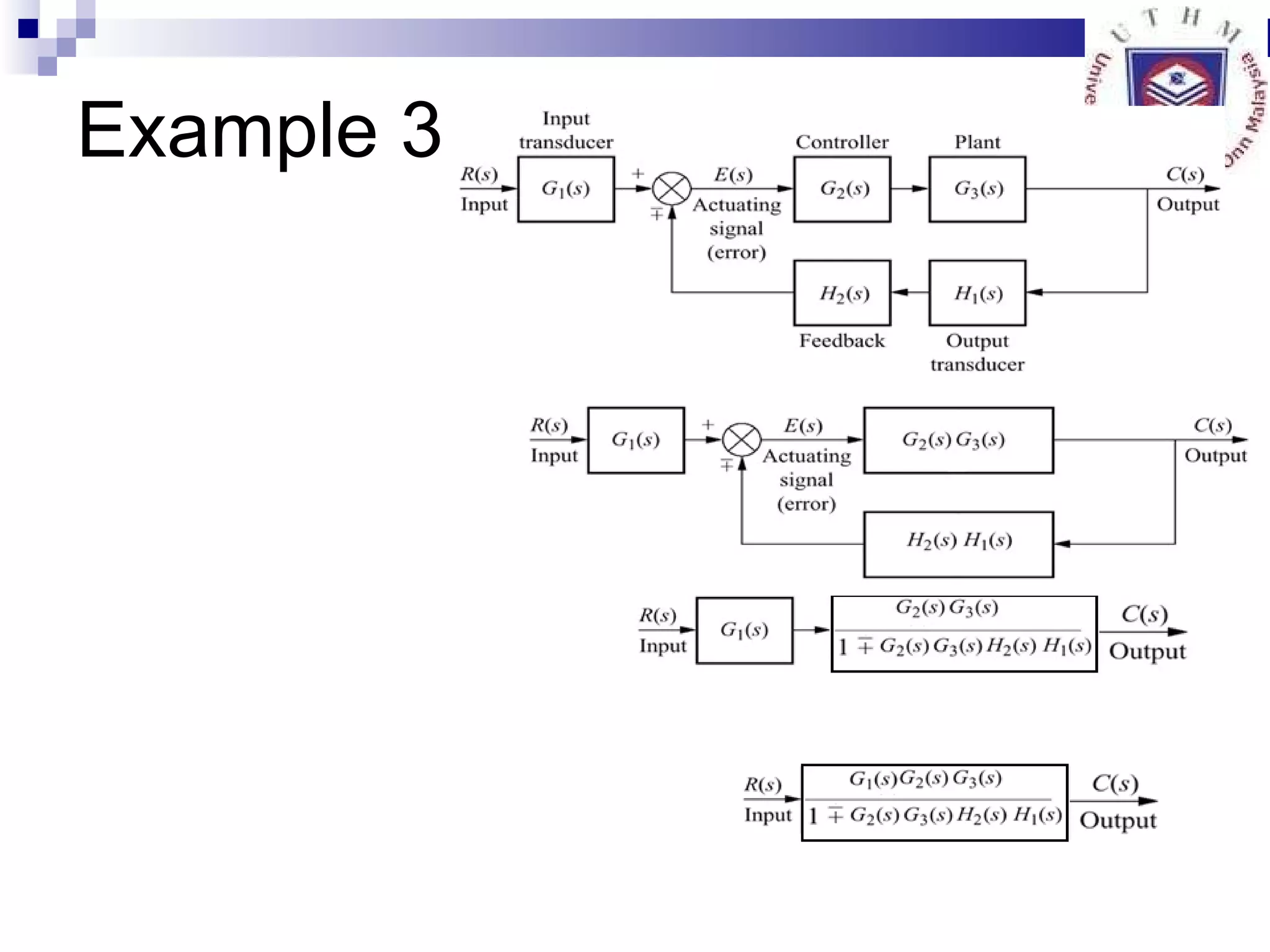
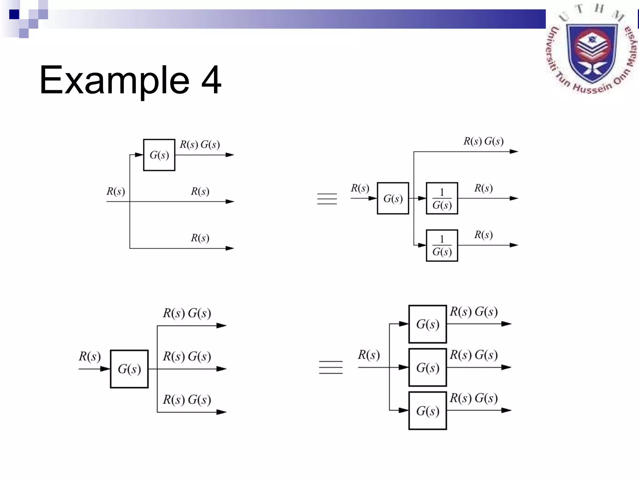
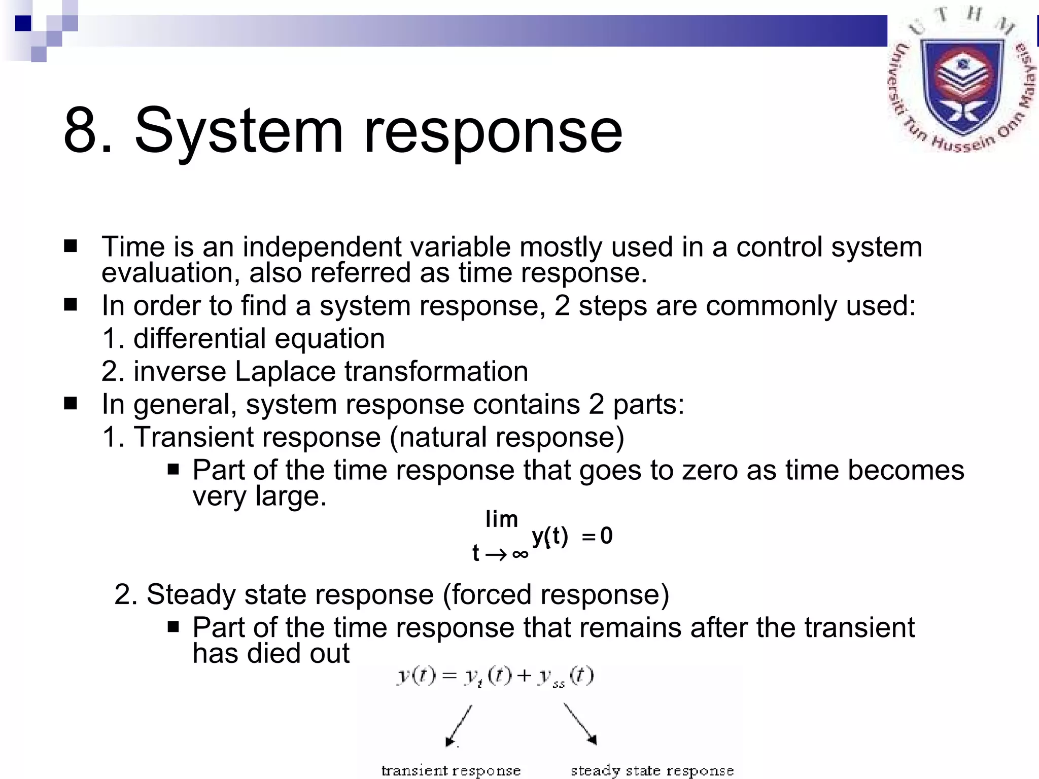
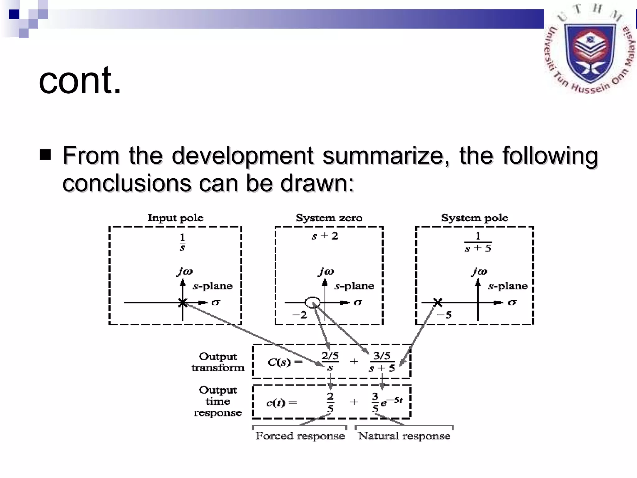
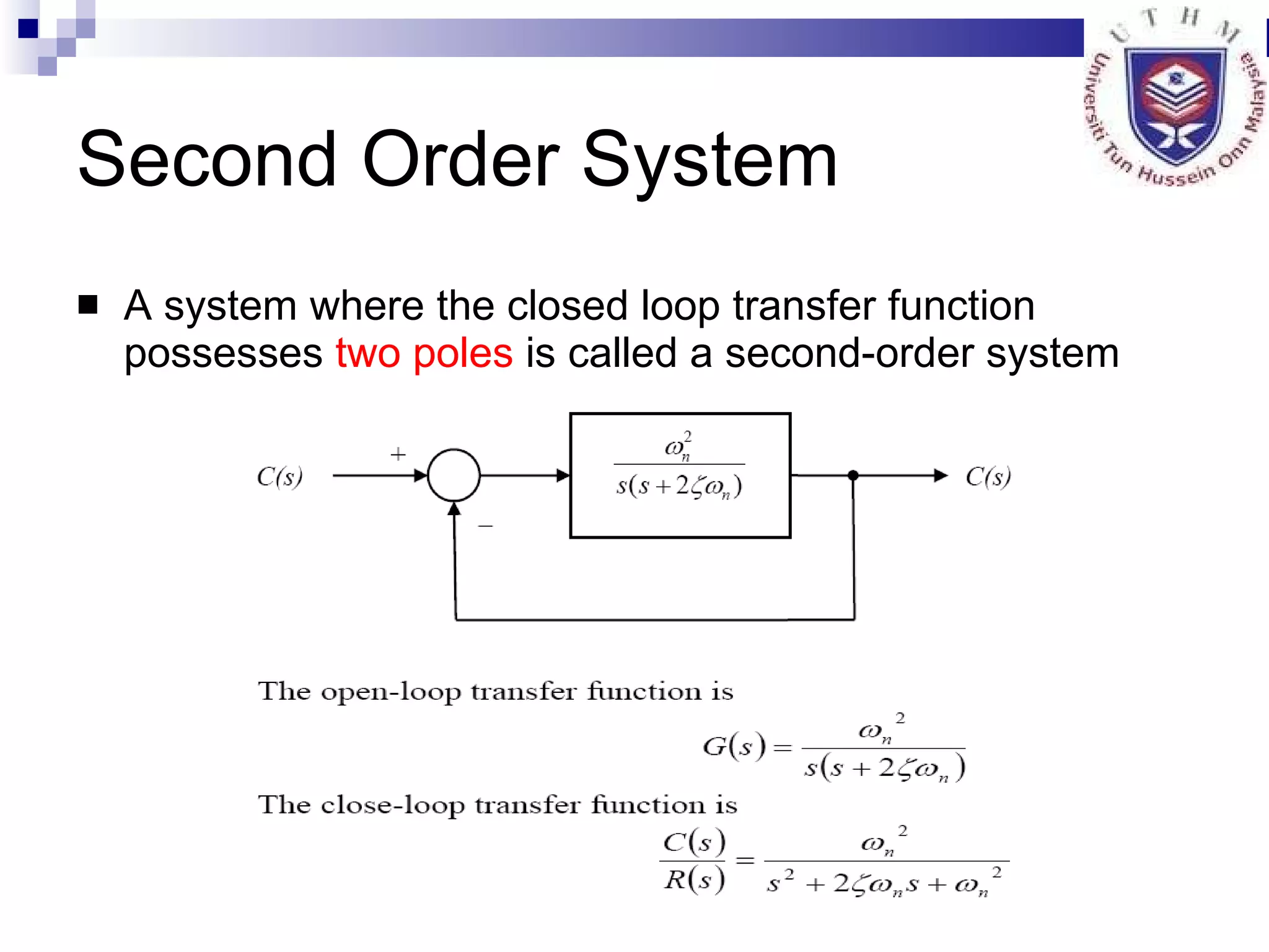
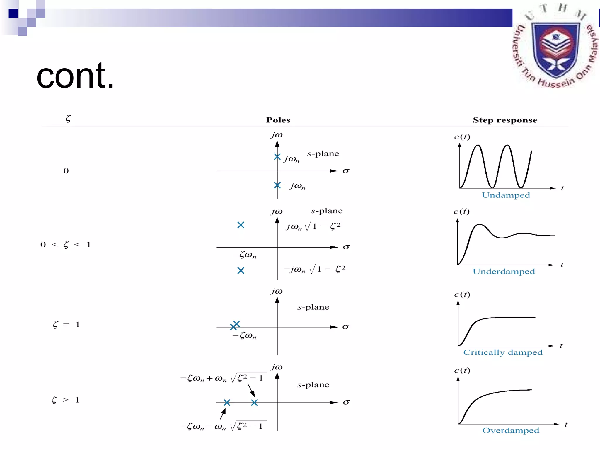
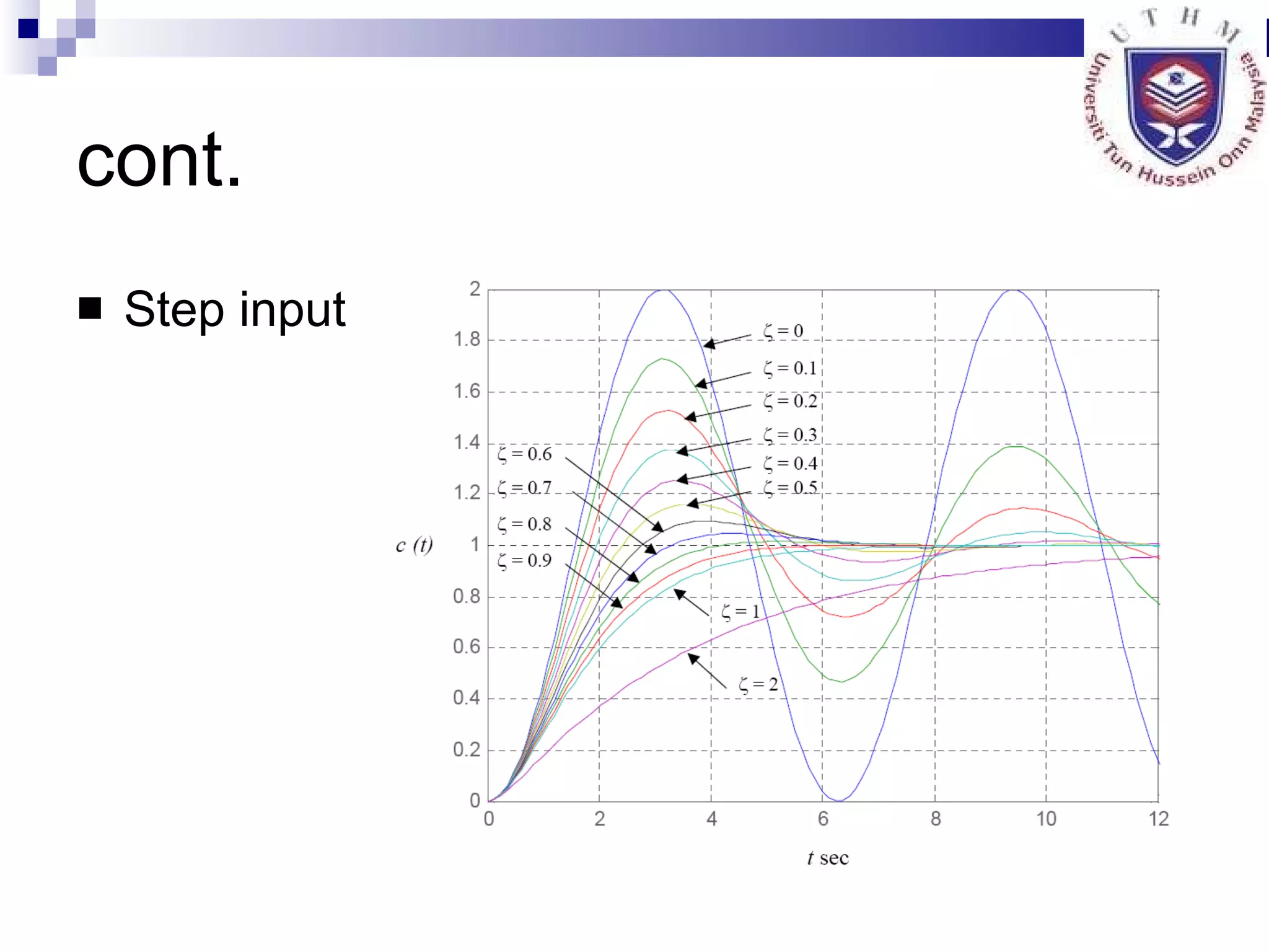
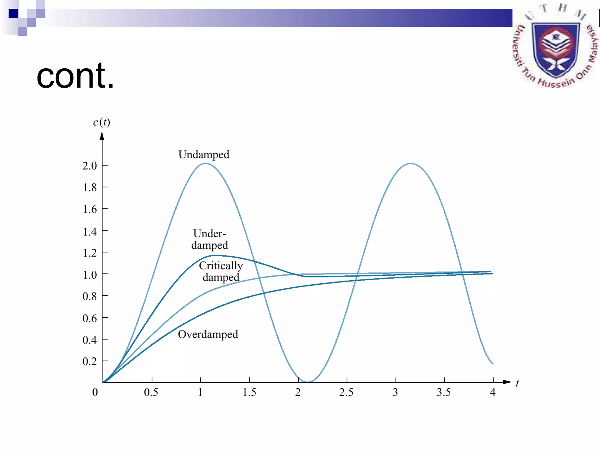
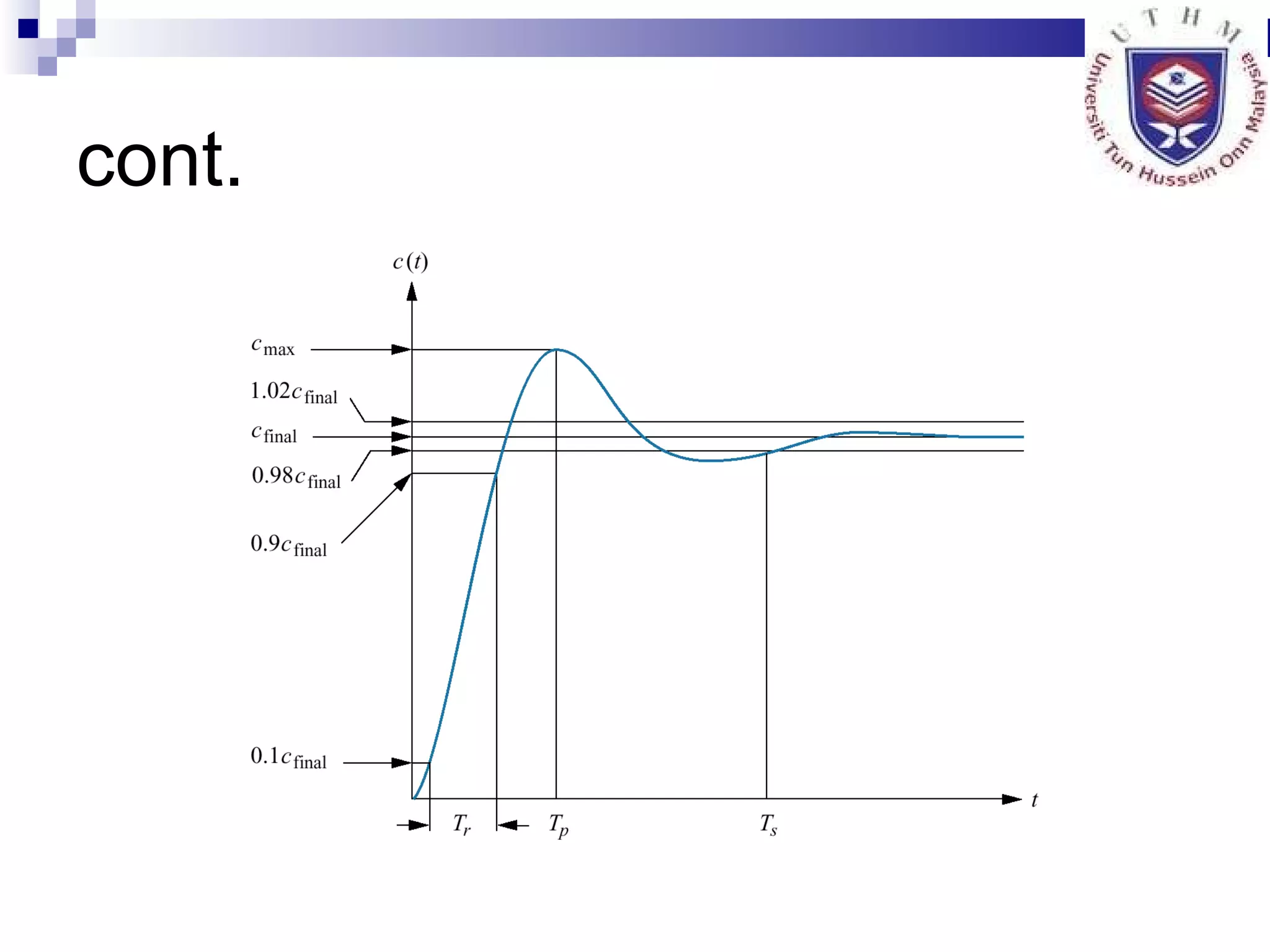
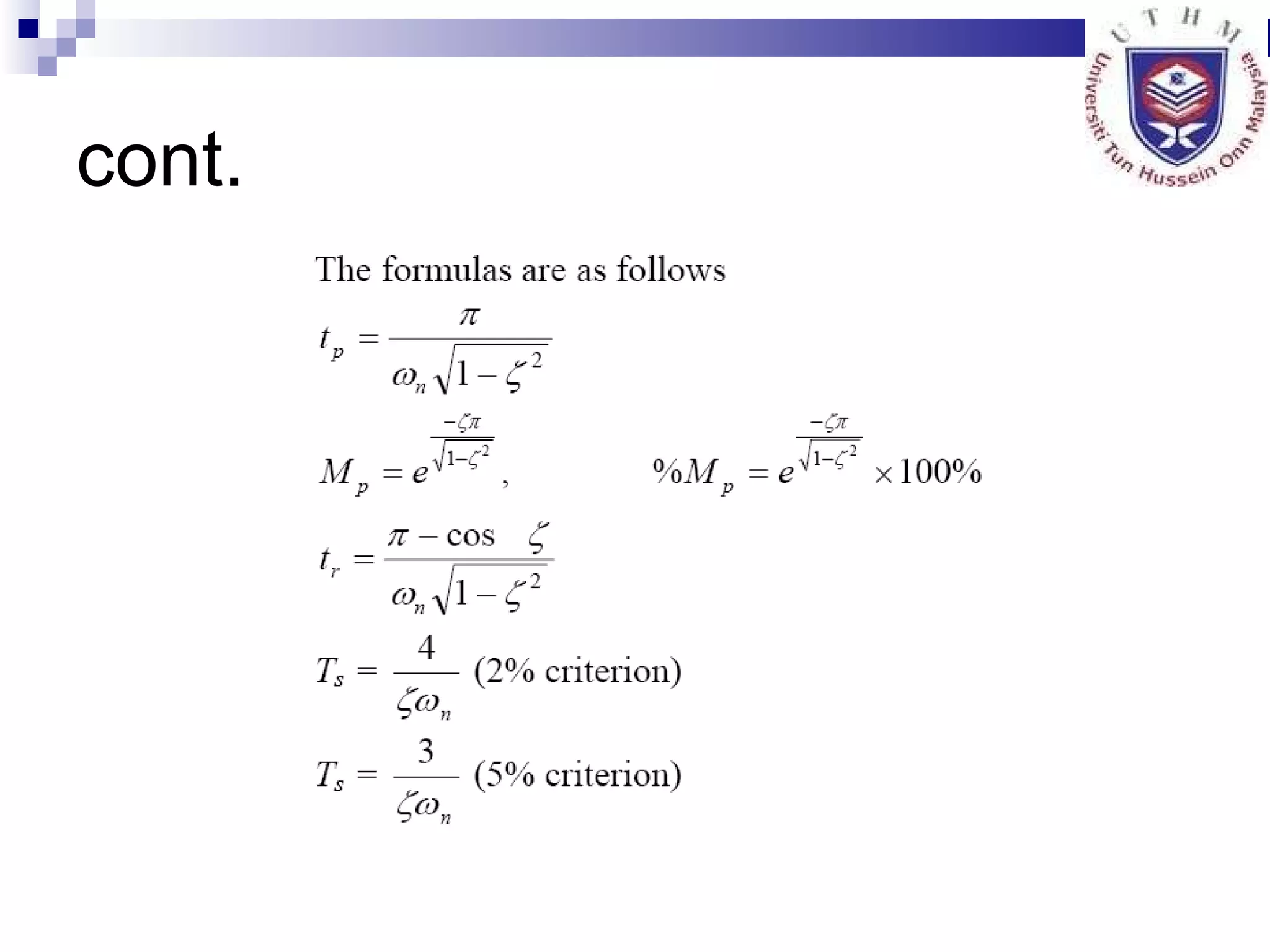
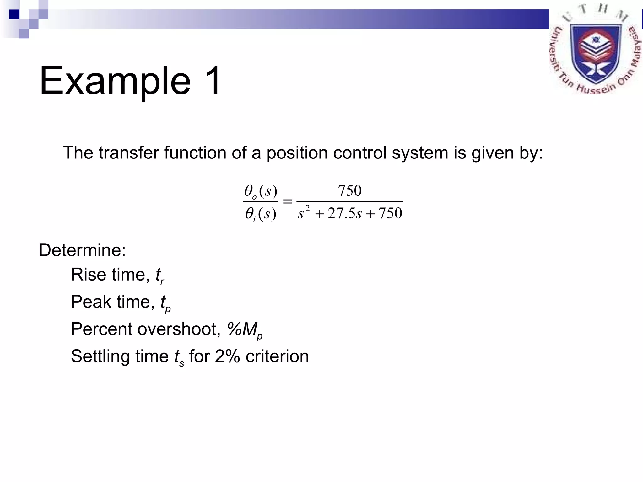
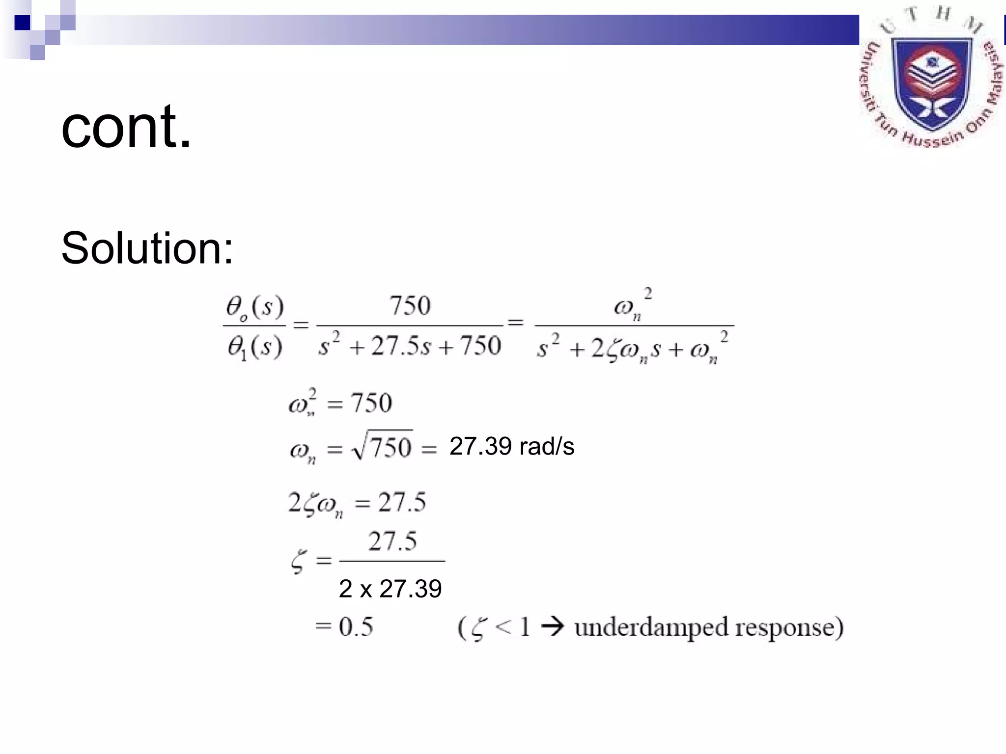
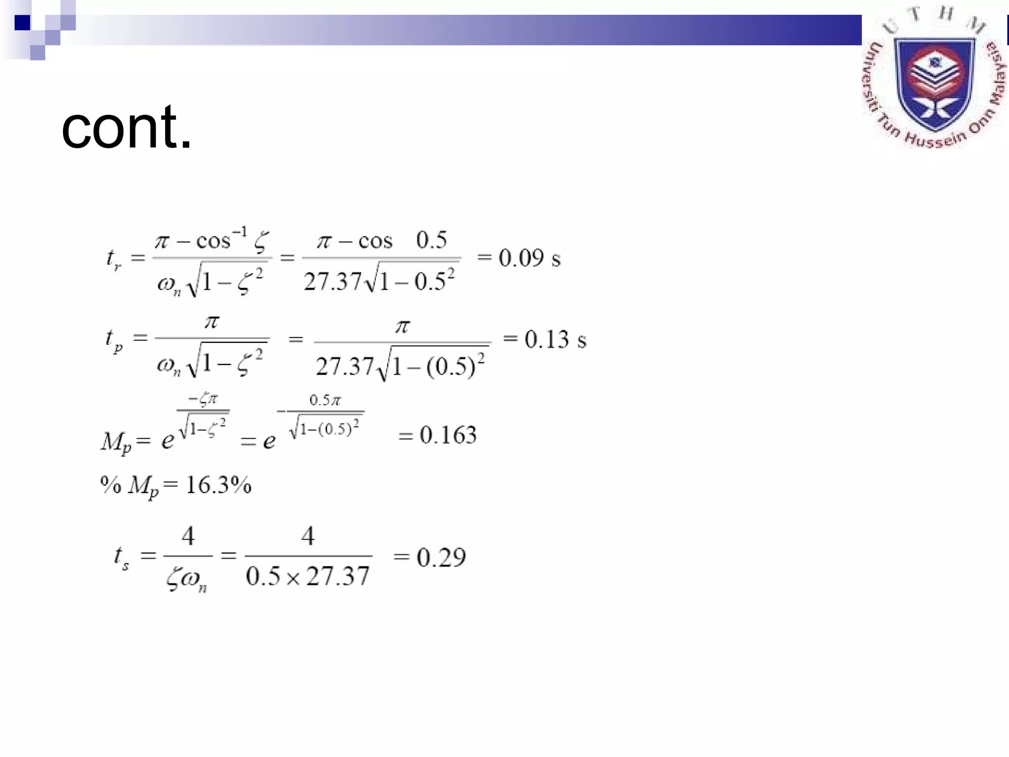
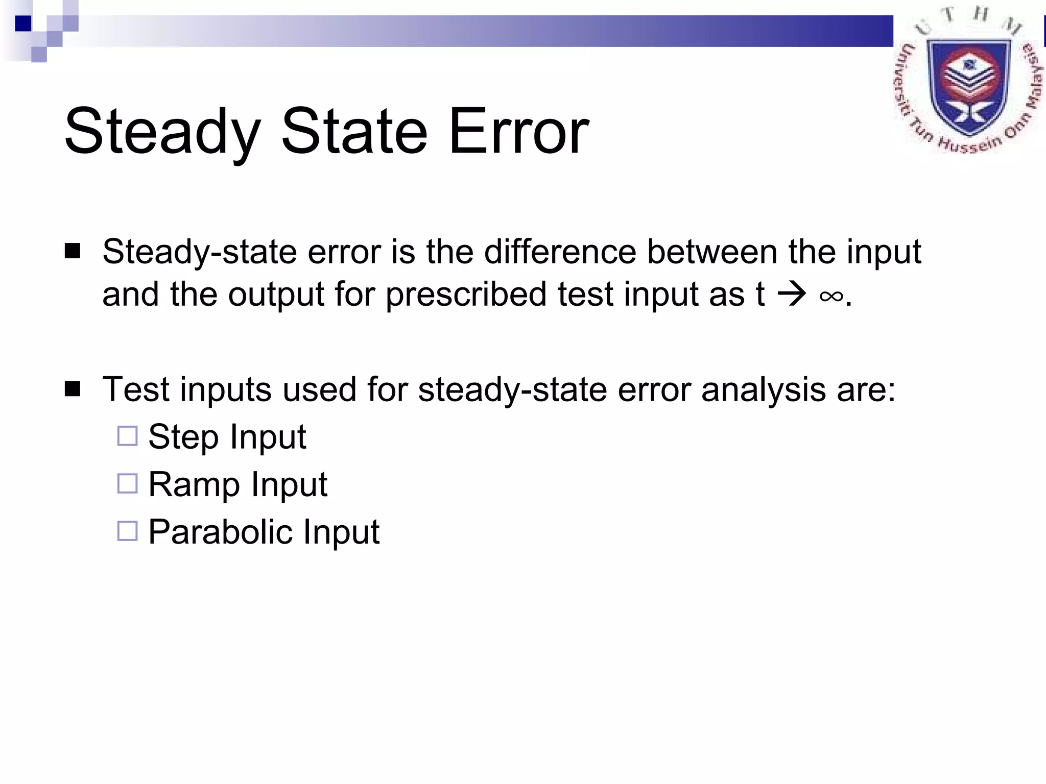
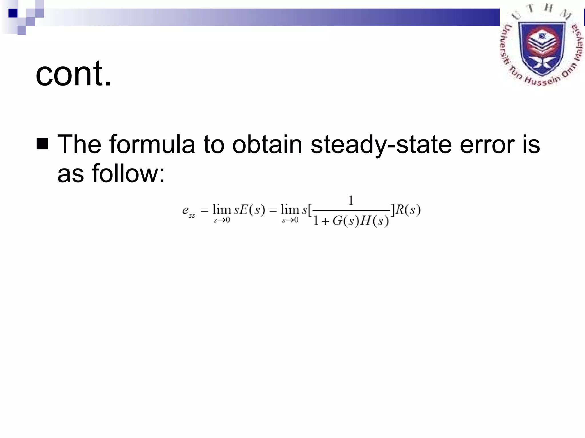
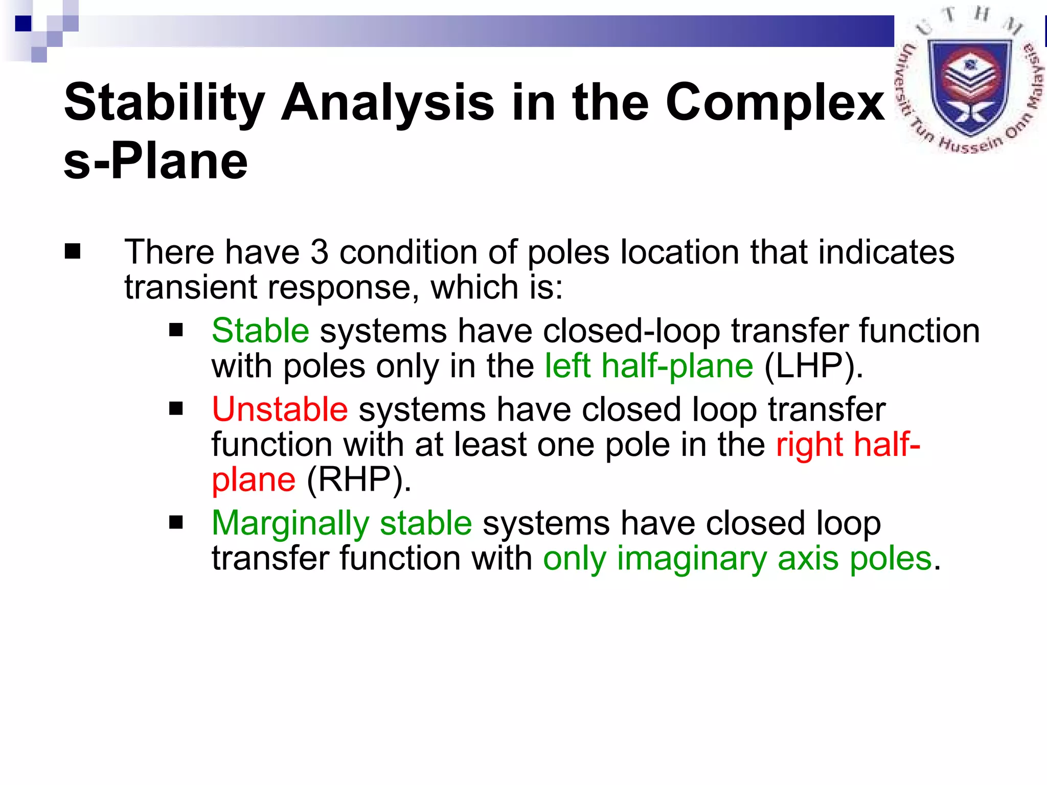
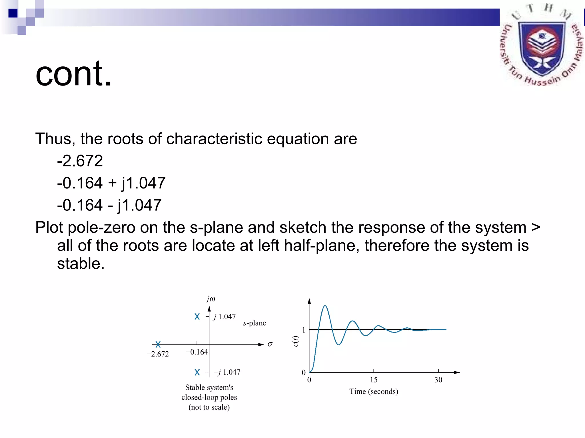
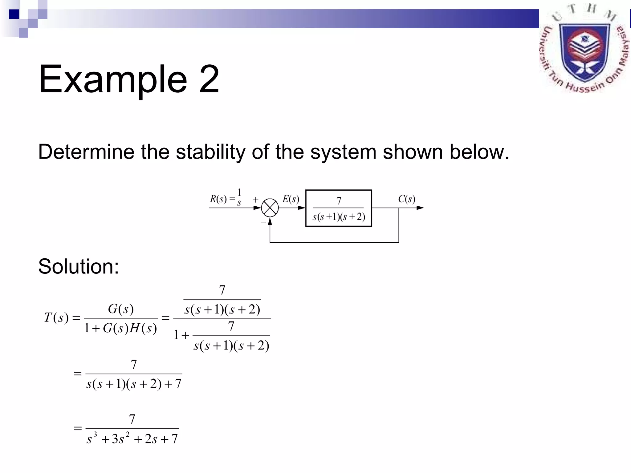
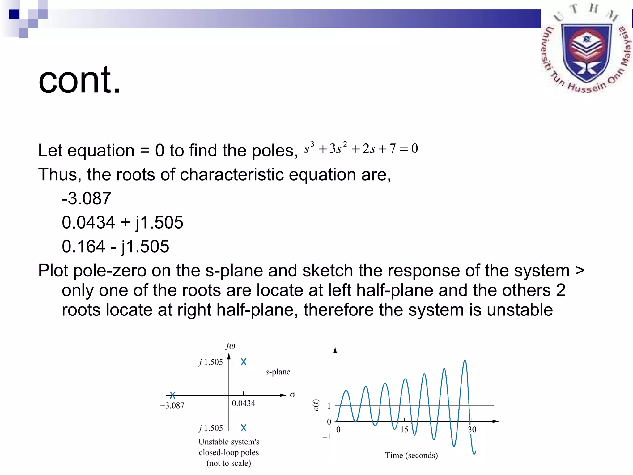
The document discusses multiple topics related to analog control systems, including: 1. Reducing multiple subsystems into a single block to simplify analysis. 2. Describing system response in terms of transient and steady state response. 3. Explaining poles, zeros and how they relate to system response. 4. Defining characteristics of second order systems and analyzing steady state error. 5. Discussing stability analysis in the complex s-plane and conditions for stable, unstable and marginally stable systems.

1. Chapter 2 – Analog Control System (cont.) Reduction of Multiple Subsystem System Response – Poles/ Zeros, Second Order System, Steady State Error, Stability Analysis

2. 7. Reduction of Multiple Subsystem Subsystem is represented as a block with an input, output and transfer function. Many systems are composed of multiple subsystems. When multiple subsystem are interconnected, new element must be added like summing junction and pickoff points. The main purpose of reduction multiple subsystem is to reduce more complicated systems to a single block.

3. Component of a block diagram for a linear, time-invariant system

5. Example 1 Cascade form

6. Example 2 Parallel form

7. Example 3

8. Example 4

9. 8. System response Time is an independent variable mostly used in a control system evaluation, also referred as time response. In order to find a system response, 2 steps are commonly used: 1. differential equation 2. inverse Laplace transformation In general, system response contains 2 parts: 1. Transient response (natural response) Part of the time response that goes to zero as time becomes very large. 2. Steady state response (forced response) Part of the time response that remains after the transient has died out

10. Example 1 Find the response of the system for a step input . Solution :

11. Poles, Zeros and System Response Poles is the values of the Laplace transform variable( s ) that cause the transfer function to become infinite or any roots of the denominator of the transfer function . Zeros is the values of the Laplace transform variable( s ) that cause the transfer function to become zero , or any roots of the numerator of the transfer function .

12. Example 1 Given the transfer function G ( s ) in Figure below, a pole exists at s = -5, and a zero exists at -2. These values are plotted on the complex s-plane, using x for the pole and О for the zero.

13. cont. Solution: To show the properties of the poles and zeros, lets applied unit step response of the system. Multiplying the transfer function by a step function yields : Thus :

14. cont. From the development summarize, the following conclusions can be drawn:

15. Second Order System A system where the closed loop transfer function possesses two poles is called a second-order system

16. cont.

17. cont. Step input

18. cont.

19. cont.

20. cont.

21. Example 1 The transfer function of a position control system is given by: Determine: Rise time, t r Peak time, t p Percent overshoot, %M p Settling time t s for 2% criterion

22. cont. Solution: 27.39 rad/s 2 x 27.39

23. cont.

24. Steady State Error Steady-state error is the difference between the input and the output for prescribed test input as t   . Test inputs used for steady-state error analysis are: Step Input Ramp Input Parabolic Input

25. cont. Figure has a step input and two possible output. Output 1 has zero steady-state error, and Output 2 has a finite steady-state error e2(  ) .

26. cont. The formula to obtain steady-state error is as follow:

27. Step input

28. Ramp Input

29. Parabolic Input

30. Stability Analysis A system is stable if every bounded input yields a bounded output . A system is unstable if any bounded input yields an unbounded output. A system is marginally stable/neutral if the system is stable for some bounded input and unstable for the others ( as undamped ) but remains constant or oscillates.

31. Stability Analysis in the Complex s-Plane There have 3 condition of poles location that indicates transient response, which is: Stable systems have closed-loop transfer function with poles only in the left half-plane (LHP). Unstable systems have closed loop transfer function with at least one pole in the right half-plane (RHP). Marginally stable systems have closed loop transfer function with only imaginary axis poles .

32. cont.

34. Example 1 Determine whether the unity feedback system below is stable or unstable. Solution: Let equation = 0 to find the poles,

35. cont. Thus, the roots of characteristic equation are -2.672 -0.164 + j1.047 -0.164 - j1.047 Plot pole-zero on the s-plane and sketch the response of the system > all of the roots are locate at left half-plane, therefore the system is stable.

36. Example 2 Determine the stability of the system shown below. Solution:

37. cont. Let equation = 0 to find the poles, Thus, the roots of characteristic equation are, -3.087 0.0434 + j1.505 0.164 - j1.505 Plot pole-zero on the s-plane and sketch the response of the system > only one of the roots are locate at left half-plane and the others 2 roots locate at right half-plane, therefore the system is unstable