Download as PDF, PPTX


![8/31/2023 Mathematics Discipline
29
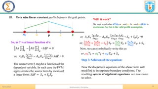
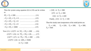
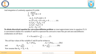
This can be rearranged to give
[(𝐷𝑊 −
𝐹𝑊
2
) + (𝐷𝑒 +
𝐹𝑒
2
)]𝑄𝑃 =(𝐷𝑊 +
𝐹𝑊
2
)𝑄𝑊 + (𝐷𝑒 −
𝐹𝑒
2
)𝑄𝐸
Or, [(𝐷𝑊 +
𝐹𝑊
2
) + 𝐷𝑒 −
𝐹𝑒
2
+ (𝐹𝑒 − 𝐹𝑤)]𝑄𝑃 =(𝐷𝑊 +
𝐹𝑊
2
)𝑄𝑊 + (𝐷𝑒 −
𝐹𝑒
2
)𝑄𝐸 … … … (14)
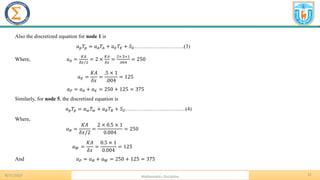
Now identifying the coefficient 𝜑𝑊 and 𝜑𝐸 as 𝑎𝑊 and 𝑎𝐸 , the central differencing expressions for the
discretized convection diffusion equations are
𝑎𝑃𝜑𝑃 = 𝑎𝑊𝜑𝑊 + 𝑎𝐸𝜑𝐸 (15)
Where
𝑎𝑊 = 𝐷𝑊 +
𝐹𝑤
2
,
𝑎𝐸 = 𝐷𝑒 +
𝐹𝑒
2
and 𝑎𝑃 = 𝑎𝑊 + 𝑎𝐸 + (𝐹𝑒 − 𝐹𝑤) (16)
Then to solve a one-dimensional convection diffusion problem we write discretized equations of the form
(15) for all grid nodes. This yields a set of algebraic equations that is solved to obtain the distribution of the
transport property 𝜑 .](https://image.slidesharecdn.com/anapresentationgroup-04-230831044425-6e32c9eb/85/Finite-Volume-Method-Advanced-Numerical-Analysis-by-Md-Al-Amin-29-320.jpg)
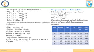


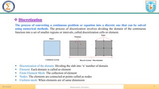
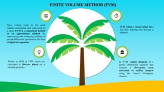
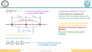
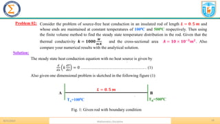
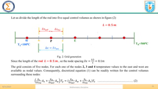
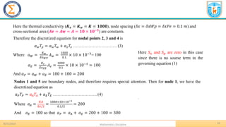
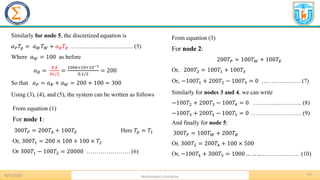
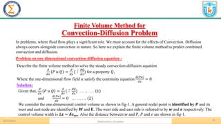
Finite volume refers to the small volume surrounding each node point on a mesh. The finite volume method (FVM) is a numerical method that converts partial differential equations into algebraic equations. FVM involves (1) grid generation by dividing the domain into control volumes, (2) discretizing the governing equations by integrating over each control volume, and (3) solving the algebraic equations. FVM follows the conservation law by ensuring flux entering and leaving each control volume is identical. The document provides an example of using FVM to solve the 1D steady state heat equation.