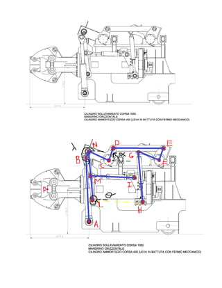
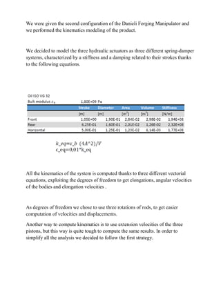
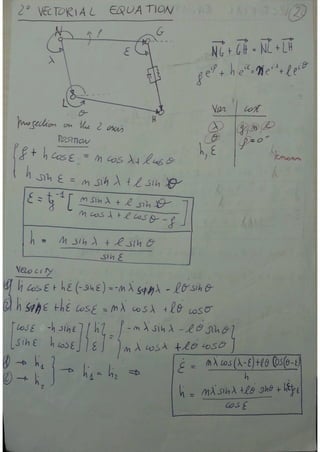
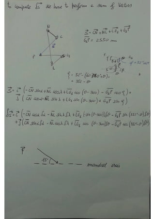
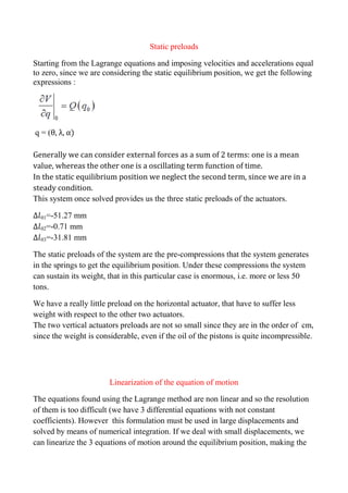
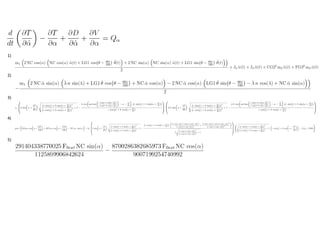
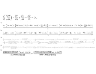
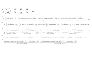
This document summarizes a mechanical engineering student project analyzing the kinematics and dynamics of a forging manipulator. It includes: 1) Modeling the hydraulic actuators as spring-damper systems and computing kinematics using vector equations of the degrees of freedom. 2) Computing static preloads on the actuators to achieve equilibrium. 3) Linearizing the equations of motion around the equilibrium position to determine natural frequencies and mode shapes. 4) Calculating frequency response functions by solving the linearized equations with an external forcing function.

1. POLITECNICO DI MILANO
Industrial Engineering department
Academic year 2013-14
Bachelor’s degree in Mechanical Engineering
Mechanical Vibrations year project
Danieli Breda Forging Manipulator
Paolo Pennacchi
Francesco Ripamonti
Authors:
Luca Bazzucchi, 773783
Filippo Campolmi, 794252
Florian Zatti, 772672

3. We were given the second configuration of the Danieli Forging Manipulator and
we performed the kinematics modeling of the product.
We decided to model the three hydraulic actuators as three different spring-damper
systems, characterized by a stiffness and a damping related to their strokes thanks
to the following equations.
All the kinematics of the system is computed thanks to three different vectorial
equations, exploiting the degrees of freedom to get elongations, angular velocities
of the bodies and elongation velocities .
As degrees of freedom we chose to use three rotations of rods, to get easier
computation of velocities and displacements.
Another way to compute kinematics is to use extension velocities of the three
pistons, but this way is quite tough to compute the same results. In order to
simplify all the analysis we decided to follow the first strategy.

11. 1)
2)
3)
4)
5)

12. 1)
2)
3)
4)
5)

13. 1)
2)
3)
4)
5)

14. Static preloads
Starting from the Lagrange equations and imposing velocities and accelerations equal
to zero, since we are considering the static equilibrium position, we get the following
expressions :
q = (θ, λ, α)
Generally we can consider external forces as a sum of 2 terms: one is a mean
value, whereas the other one is a oscillating term function of time.
In the static equilibrium position we neglect the second term, since we are in a
steady condition.
This system once solved provides us the three static preloads of the actuators.
01=-51.27 mm
02=-0.71 mm
03=-31.81 mm
The static preloads of the system are the pre-compressions that the system generates
in the springs to get the equilibrium position. Under these compressions the system
can sustain its weight, that in this particular case is enormous, i.e. more or less 50
tons.
We have a really little preload on the horizontal actuator, that have to suffer less
weight with respect to the other two actuators.
The two vertical actuators preloads are not so small since they are in the order of cm,
since the weight is considerable, even if the oil of the pistons is quite incompressible.
Linearization of the equation of motion
The equations found using the Lagrange method are non linear and so the resolution
of them is too difficult (we have 3 differential equations with not constant
coefficients). However this formulation must be used in large displacements and
solved by means of numerical integration. If we deal with small displacements, we
can linearize the 3 equations of motion around the equilibrium position, making the

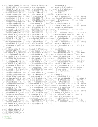
15. solution of the system easier. So we will linearize the 4 contributions (potential
energy, dissipative function, kinetic energy and Q) of the Lagrange equations.
Linearization of potential energy V
For a one degree of freedom system the approach is the following one: we perform
the Taylor expansion of around the equilibrium position ( q=q0) , finding its first
order term which is the equivalent stiffness of the linearized system in small
displacements; this procedure returns two contributions:
Elastic contribution :
Gravitational contribution :
The total equivalent stiffness is simply the sum of these 2 quantities.
For a multidegree of freedom system, as in our case, the procedure is the same; the
only difference is that we have matrices instead of scalar values.
V= zT
[K] z;
The equivalent stiffness matrix becomes:

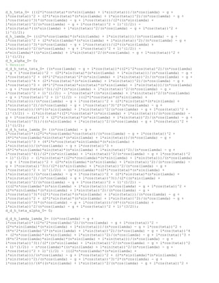
16. Where:
 i=1,2,3 (there are 3 actuators);
 ki is the stiffness of each actuator;
 mi is the mass of each body;
 KF is a diagonal matrix containing the 3 actuator stiffnesses ;
 Yk is a vector containing the 3 elongations 1, 2, 3;
 Jk is the stiffness jacobian;
 H is the hessian matrix;
 0 is the static preload of the actuators.
Jk θ λ α
1 0 0 1134.3
2 -1162.3 1162.3 0
3 -2477.4 -14.3 0
HΔl1 = [ ]
H Δl2 = [ ]
H Δl3 = [ ]
Hhg1 = 1.0e+03 * [ ]

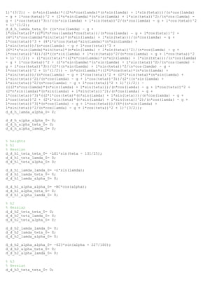
17. Hhg2 = [ ]
Hhg3 = [ ]
K_el_I = 1.0e+12 * [ ] N/m
K_el_II = 1.0e+09 * [ ] N/m
K_g = 1.0e+08 * [ ] N/m
[K]=[ K_el_I] + [K_el_II] + [K_g] =1.0e+12*[ ] N/m
Linearization of dissipative function D
The dissipative function for a multidegree of freedom system is: D = ̇k
T
[RF] ̇k ,
where:
 ̇k is a vector containing the elongation velocities of the 3 actuators;
 [RF] is a diagonal matrix containing the damping coefficients of the 3
actuators.

18. Since ̇k = [Jk] zT
(Jk is the stiffness jacobian), D becomes:
D = ̇T
[R] ̇ with [R] = [Jk]T
[RF] [Jk];
[R]= 1.0e+10 * [ ] (N*s)/m
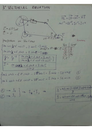
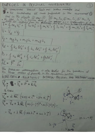
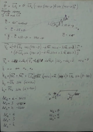
Linearization of kinetic energy T
In order to perform the linearization of the kinetic energy, we have linearized the
kinematic relationships getting the following results:
V1x - ̇ LG1 cos(6.81-θo) - ̇ NC cos(αo) - ̇ n sin(λo)
V1y ̇ LG1 sin(6.81-θo) - ̇ NC sin(αo) + ̇ n cos(λo)
ω1 ̇
V2 CG2 α̇
ω2 ̇
V3 FG3 α̇
θo, αo and λo are the values of the independent coordinates θ, λ, α at the
equilibrium position.
(V1)2
= (V1x)2
+ (V1y)2
We have projected the velocity V1 on x and y direction to get an easier matrix
representation in the mass jacobian.

19. Mass jacobian
JM ̇ ̇ ̇
V1x -564.6 -408.8 2291.2
V1y 369.9 -1021.2 201.2
ω1 0 0 623.0
V2 0 0 467.0
ω2 1 0 0
V3 0 0 1
ω3 0 0 1
The kinetic energy for a multidegree of freedom system is: T= ̇M
T
[MF] ̇M
where:
 ̇M is a vector containing all the velocities of the bodies in physical
coordinates;
 [MF] is a diagonal matrix containing masses and inertia properties of the 3
bodies; since we have considered V1x and V1y, MF becomes diag ( m1, m1, J1,
m2, J2, m3, J3 );
Since ̇M = [JM] ̇, T becomes: T = ̇T
[M] ̇ with [M] = [JM]T
[MF] [JM]; [M] is the
mass matrix.
[M] = 1.0e+11 [ ] kg

20. Linearization of lagrangian component Q
In general an external force F(t) having non null average value can be written as the
sum of two contributions:
 ̅ mean value;
 ̃(t) oscillatory component.
For a single degree of freedom system the general expression of the Lagrangian
component of the external force is:
where:
The first step we have performed is to project s (virtual displacement of the point in
which the force is applied) on x and y direction and then we have linearized the
kinematic relationships: as a consequence, the fourth expression (“equivalent
stiffness Mathieu-like”) and the third one are null. Since the oscillatory component is

21. not present in our external force, even the second term is null. So the only term that
remains is the first one.
For a multidegree of freedom system the previous considerations are still valid; the
difference is that:
*
L = F
T
F = zT
( [JM] T
F ) = zT
QF
where:
F {
s
s } F = { } z = {
θ
λ
α
}
[JM] is the force jacobian:
JM θ λ α
sx -335.1 2291.2 -408.8
sy -2169.3 -201.2 -1021.2
Natural frequencies and mode shapes
Once we have linearized T, D, V and Q, we apply the Lagrange method and we
obtain three linearized equations of motion.
[M] ̈ + [R] ̇ + [K] z = Q
These equations are coupled; this means that
 from the mathematical point of view, we can not start solving one equation
independently from the other;
 from the physical point of view, the motion of a certain mass will influence the
motion of the other ones.
Now we can solve the system and find the solution. The first step is to calculate the
natural frequencies. To do this, we will consider the unforced and undamped system:
[M] ̈ + [K] z = 0

22. Its solution will be: z = z0 eiωt
z0 = {
̃
̃
̃
}
Deriving z with respect to time, we obtain: ̇ = iωz0 eiωt
; ̈ = -ω2
z0 eiωt
Substituting these terms inside the system:
( -ω2
[M] + [K] ) z0 eiωt
= 0
since this expression must be satisfied for all values of time t
( -ω2
[M] + [K] ) z0 = 0
This is an algebraic system in which the unknown is z0. If the determinant of the
coefficients matrix is different from zero, there will be only one solution, that will be
the trivial one since this system is also homogenous.
Trivial solution means {
̃
̃
̃
} = { } no vibration !!!
In order to avoid this situation, we must impose that the determinant of the
coefficients matrix is equal to zero and so we obtain an equation called “frequencies
or characteristic equation” in which the unknown is ω.
̃, ̃, ̃ are the
amplitudes of the θ, λ, α
respectively

23. Solving this equation, we obtain the natural frequencies of our system:
ω1 = 27.3928 rad/s ω2 = 2.7260 rad/s ω3 = 1.0936 rad/s
We could have used another procedure in order to get the natural frequencies:
( -ω2
[M] + [K] ) z0 = 0
-ω2
[I] + [M]-1
[K]
[A]
So we obtain: ω2
[I] z0 = [A] z0
[φ] = [ ]
Observation: z = [φ] q
This is an eigenvalue problem in which:
 ω are the eigenvalues;
 the eigenvectors are collected in a
matrix called “φ” (mode shapes).
q is the vector containing
the modal coordinates

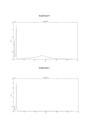
24. Frequency response function
We will start from the linearize equations of motion ( [M] ̈ + [R] ̇ + [K] z = Q ) and
we will suppose that the external force is F = F0 e iΩt
(approach with complex
numbers).
Q = Q0 e iΩt
z = z0 eiΩt
Deriving z with respect time, we obtain:
̇ =iΩz0eiΩt
; ̈ = -Ω2
z0 eiΩt
This is the
particular
solution

25. Substituting these terms inside the system:
( -Ω2
[M] + i Ω [R] + [K] ) z0 eiωt
= Q0 e iΩt
( -Ω2
[M] + i Ω [R] + [K] ) z0= Q0
[A]=[A(Ω)]
So: z0= [A]-1
Q0.
an amplitude
z0 is a complex number and hence it has
a phase
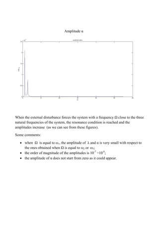
In the following pictures, we have considered Ω = [ 0 … 2*ω1].
Matrix of the
mechanical
impedence of the
system

26. Amplitude θ
Amplitude λ

27. Amplitude α
When the external disturbance forces the system with a frequency Ω close to the three
natural frequencies of the system, the resonance condition is reached and the
amplitudes increase (as we can see from these figures).
Some comments:
 when Ω is equal to ω1, the amplitude of λ and α is very small with respect to
the ones obtained when Ω is equal to ω2 or ω3;
 the order of magnitude of the amplitudes is 10-7
÷10-8
;
 the amplitude of α does not start from zero as it could appear.

28. Phase θ
Phase λ

29. Phase α
When we are in the resonance condition, the phase is (as it should be).
From the previous considerations, we can state the these pictures are reasonable and
compatible with the theory we have studied and the system we dealt with.

30. Lagrange’ equations
clc
clear all
close all
syms k1 k2 k3 c csi b alpha teta lamda m l I_1 n g m1 m2 m3 J1 J2 J3 grav NC LG1 CG2
FG3 PG1 delta_1_static delta_2_static delta_3_static c1 c2 c3 lamda_dot teta_dot
alpha_dot F0_ext de_alpha de_teta de_lamda
%%%%% potential energy eventualmente correggere lamBa
% delta_1
alpha_tilde=alpha+1.85;
eta= atan( (c*sin(csi)+b*sin(alpha_tilde)) / (c*cos(csi)+b*cos(alpha_tilde)) ) + pi ;
% attenzione all'arcotangente!!! va aggiunto "pi"
a= (c*cos(csi)+b*cos(alpha_tilde)) / cos(eta);
delta_1_dynamic= -3025 + a; % dinamico
delta_1= delta_1_dynamic+delta_1_static;
% delta_2
tau=teta-4.31;
gamma= atan( (m*sin(lamda)+l*sin(teta)+I_1*sin(tau)) /
(m*cos(lamda)+l*cos(teta)+I_1*cos(tau)) );
j= (m*sin(lamda)+l*sin(teta)+I_1*sin(tau)) / sin(gamma);
delta_2_dynamic= j-2175;
delta_2= delta_2_dynamic+delta_2_static;
% delta_3
epsilon= atan( (n*sin(lamda)+l*sin(teta)) / (n*cos(lamda)+l*cos(teta)-g) );
h= (n*sin(lamda)+l*sin(teta)) / sin(epsilon);
delta_3_dynamic= h-2400;
delta_3= delta_3_dynamic+delta_3_static;
% elastic potential energy
V_el=0.5* ( k1*(delta_1)^2 + k2*(delta_2)^2 + k3*(delta_3)^2 );
% height 1
h1= NC*cos(alpha)+n*sin(lamda)+LG1*sin(teta-5.24);
% height 2
h2= 623*sin(alpha+2.27);
% height 3
h3= 467*sin(alpha+2.79);
% gravitational potential energy
V_g= grav*(m1*h1+m2*h2+m3*h3);
V=V_el+V_g;
%%%%% dissipative function
% delta_1_dot
eta_dot= b*alpha_dot*cos(alpha_tilde-eta)/a;
a_dot= (-b*alpha_dot*sin(alpha_tilde) / cos(eta) )+ a*eta_dot*tan(eta);

31. delta_1_dot=a_dot;
% delta_2_dot
gamma_dot= (m*lamda_dot*cos(lamda-gamma)+teta_dot*( l*cos(teta-gamma)+I_1*cos(tau-
gamma))) / j;
j_dot= (m*lamda_dot*cos(lamda)+l*teta_dot*cos(teta)+I_1*teta_dot*cos(tau)) / sin(gamma)
- j*gamma_dot*cot(gamma);
delta_2_dot=j_dot;
% delta_3_dot
epsilon_dot= (n*lamda_dot*cos(lamda-epsilon)+l*teta_dot*cos(teta-epsilon)) / h;
h_dot= (n*lamda_dot*sin(lamda)+l*teta_dot*sin(teta)) / cos(epsilon) +
h*epsilon_dot*tan(epsilon);
delta_3_dot= h_dot;
D= 0.5* ( c1*delta_1_dot^2 + c2*delta_2_dot^2 + c3*delta_3_dot^2 );
%%%%% kinetic energy
% velocities
v1x= -teta_dot*LG1*cos(6.81-teta)-alpha_dot*NC*cos(alpha)-lamda_dot*n*sin(lamda);
v1y= teta_dot*LG1*sin(6.81-teta)-alpha_dot*NC*sin(alpha)+lamda_dot*n*cos(lamda);
v1= sqrt(v1x^2 + v1y^2);
v2= CG2*alpha_dot;
v3= FG3*alpha_dot;
% angular speed
omega_1= teta_dot;
omega_2= alpha_dot;
omega_3= alpha_dot;
T= 0.5*( m1*v1^2 + m2*v2^2 + m3*v3^2 +J1*omega_1^2 + J2*omega_2^2 + J3*omega_3^2 );
%%%%% virtual work % angles in degrees!!!!!!!!!!!!!!!
F_ext_x= F0_ext*cosd(15);
F_ext_y= -F0_ext*sind(15);
de_s_x= -NC*cos(alpha)*de_alpha - n*sin(lamda)*de_lamda - LG1*sin(teta-5.24)*de_teta -
PG1*sin(6.14-teta)*de_teta;
de_s_y= -NC*sin(alpha)*de_alpha - n*cos(lamda)*de_lamda + LG1*cos(teta-5.24)*de_teta -
PG1*cos(6.14-teta)*de_teta;
de_work= F_ext_x*de_s_x + F_ext_y*de_s_y; % da derivare rispetto ai de_...
%%%%% derivatives
% derivative of potential energy
d_V_teta= diff(V,teta);
d_V_lamda= diff(V,lamda);
d_V_alpha= diff(V,alpha);
% derivative of dissipative function
d_D_teta_dot= diff(D,teta_dot);
d_D_lamda_dot= diff(D,lamda_dot);
d_D_alpha_dot= diff(D,alpha_dot);
% derivative of de_work
Q_teta= diff(de_work,de_teta);

32. Q_lamda= diff(de_work,de_lamda);
Q_alpha= diff(de_work,de_alpha);
% derivative of kinetic energy
d_T_teta= diff( T,teta );
d_T_lamda= diff( T,lamda );
d_T_alpha= diff( T,alpha );
d_T_teta_dot= diff( T,teta_dot );
d_T_lamda_dot= diff( T,lamda_dot );
d_T_alpha_dot= diff( T,alpha_dot );
%%
clc
clear all
close all
syms t k1 k2 k3 c csi teta alpha lamda lamba_dot(t) alpha_dot(t) teta_dot(t) b m l I_1
n g m1 m2 m3 J1 J2 J3 grav NC LG1 CG2 FG3 PG1 delta_1_static delta_2_static
delta_3_static c1 c2 c3 lamda_dot teta_dot alpha_dot F0_ext de_alpha de_teta de_lamda
d_T_teta_dot=J1*teta_dot + (m1*(2*LG1*cos(teta - 681/100)*(lamda_dot*n*sin(lamda) +
LG1*teta_dot*cos(teta - 681/100) + NC*alpha_dot*cos(alpha)) + 2*LG1*sin(teta -
681/100)*(LG1*teta_dot*sin(teta - 681/100) - lamda_dot*n*cos(lamda) +
NC*alpha_dot*sin(alpha))))/2;
d_T_lamba_dot=(m1*(2*n*sin(lamda)*(lamda_dot*n*sin(lamda) + LG1*teta_dot*cos(teta -
681/100) + NC*alpha_dot*cos(alpha)) - 2*n*cos(lamda)*(LG1*teta_dot*sin(teta - 681/100)
- lamda_dot*n*cos(lamda) + NC*alpha_dot*sin(alpha))))/2;
d_T_alpha_dot=alpha_dot*m2*CG2^2 + alpha_dot*m3*FG3^2 + J2*alpha_dot + J3*alpha_dot +
(m1*(2*NC*cos(alpha)*(lamda_dot*n*sin(lamda) + LG1*teta_dot*cos(teta - 681/100) +
NC*alpha_dot*cos(alpha)) + 2*NC*sin(alpha)*(LG1*teta_dot*sin(teta - 681/100) -
lamda_dot*n*cos(lamda) + NC*alpha_dot*sin(alpha))))/2;
% derivative of kinetic energy with respect of time
d_T_teta_dot_t = diff ( d_T_teta_dot,t );
d_T_lamda_dot_t = diff ( d_T_lamba_dot,t );
d_T_alpha_dot_t = diff ( d_T_alpha_dot,t );
Linearization
clc
clear all
close all

33. syms k1 k2 k3 c csi b alpha teta lamda m l I_1 n g m1 m2 m3 J1 J2 J3 grav NC LG1 CG2
FG3 PG1 delta_1_static delta_2_static delta_3_static c1 c2 c3 lamda_dot teta_dot
alpha_dot F0_ext de_alpha de_teta de_lamda
%%%%% potential energy
% delta_1
alpha_tilde=alpha+1.85;
eta= atan( (c*sin(csi)+b*sin(alpha_tilde)) / (c*cos(csi)+b*cos(alpha_tilde)) );
a= (c*cos(csi)+b*cos(alpha_tilde)) / cos(eta);
delta_1_dynamic= -3025 + a; % dinamico
delta_1= delta_1_dynamic+delta_1_static;
% delta_2
tau=teta-4.31;
gamma= atan( (m*sin(lamda)+l*sin(teta)+I_1*sin(tau)) /
(m*cos(lamda)+l*cos(teta)+I_1*cos(tau)) );
j= (m*sin(lamda)+l*sin(teta)+I_1*sin(tau)) / sin(gamma);
delta_2_dynamic= j-2175;
delta_2= delta_2_dynamic+delta_2_static;
% delta_3
epsilon= atan( (n*sin(lamda)+l*sin(teta)) / (n*cos(lamda)+l*cos(teta)-g) );
h= (n*sin(lamda)+l*sin(teta)) / sin(epsilon);
delta_3_dynamic= h-2400;
delta_3= delta_3_dynamic+delta_3_static;
% elastic potential energy
V_el=0.5* ( k1*(delta_1)^2 + k2*(delta_2)^2 + k3*(delta_3)^2 );
% height 1
h1= NC*cos(alpha)+n*sin(lamda)+LG1*sin(teta-5.24);
% height 2
h2= 623*sin(alpha+2.27);
% height 3
h3= 467*sin(alpha+2.79);
% gravitational potential energy
V_g= grav*(m1*h1+m2*h2+m3*h3);
V=V_el+V_g;
%%%%% dissipative function
% delta_1_dot
eta_dot= b*alpha_dot*cos(alpha_tilde-eta)/a;
a_dot= (-b*alpha_dot*sin(alpha_tilde) / cos(eta) )+ a*eta_dot*tan(eta);
delta_1_dot=a_dot;
% delta 2
gamma_dot= (m*lamda_dot*cos(lamda-gamma)+teta_dot*( l*cos(teta-gamma)+I_1*cos(tau-
gamma))) / j;
j_dot= (m*lamda_dot*cos(lamda)+l*teta_dot*cos(teta)+I_1*teta_dot*cos(tau)) / sin(gamma)
- j*gamma_dot*cot(gamma);
delta_2_dot=j_dot;
% delta 3

34. epsilon_dot= (n*lamda_dot*cos(lamda-epsilon)+l*teta_dot*cos(teta-epsilon)) / h;
h_dot= (n*lamda_dot*sin(lamda)+l*teta_dot*sin(teta)) / cos(epsilon) +
h*epsilon_dot*tan(epsilon);
delta_3_dot= h_dot;
D= 0.5* ( c1*delta_1_dot^2 + c2*delta_2_dot^2 + c3*delta_3_dot^2 );
%%%%% kinetic energy
% velocities
v1x= -teta_dot*LG1*cos(6.81-teta)-alpha_dot*NC*cos(alpha)-lamda_dot*n*sin(lamda);
v1y= teta_dot*LG1*sin(6.81-teta)-alpha_dot*NC*sin(alpha)+lamda_dot*n*cos(lamda);
v1= sqrt(v1x^2 + v1y^2);
v2= CG2*alpha_dot;
v3= FG3*alpha_dot;
% angular speed
omega_1= teta_dot;
omega_2= alpha_dot;
omega_3= alpha_dot;
T= 0.5*( m1*v1^2 + m2*v2^2 + m3*v3^2 +J1*omega_1^2 + J2*omega_2^2 + J3*omega_3^2 );
%%%%% virtual work
F_ext_x= F0_ext*cosd(15);
F_ext_y= -F0_ext*sind(15);
de_s_x= -NC*cos(alpha)*de_alpha - n*sin(lamda)*de_lamda - LG1*sin(teta-5.24)*de_teta -
PG1*sin(6.14-teta)*de_teta;
de_s_y= -NC*sin(alpha)*de_alpha - n*cos(lamda)*de_lamda + LG1*cos(teta-5.24)*de_teta -
PG1*cos(6.14-teta)*de_teta;
de_work= F_ext_x*de_s_x + F_ext_y*de_s_y;
%%%%% derivatives
% derivative of potential energy
d_V_teta= diff(V,teta);
d_V_lamda= diff(V,lamda);
d_V_alpha= diff(V,alpha);
% derivative of dissipative function
d_D_teta_dot= diff(D,teta_dot);
d_D_lamda_dot= diff(D,lamda_dot);
d_D_alpha_dot= diff(D,alpha_dot);
% derivative of de_work
Q_teta= diff(de_work,de_teta);
Q_lamda= diff(de_work,de_lamda);
Q_alpha= diff(de_work,de_alpha);
%%%%%%%%%%%%%%%%%%%%%%%%%%%%%%%%%%%%%%%%%%%%%%%%%%%
%%%%% Linearization of kinematics

35. % delta_1
% Jacobian
d_a_teta= diff(a,teta);
d_a_lamda= diff(a,lamda);
d_a_alpha= diff(a,alpha);
% Hessian
d_d_a_teta_teta= diff( d_a_teta,teta );
d_d_a_teta_lamda= diff( d_a_teta,lamda );
d_d_a_teta_alpha= diff( d_a_teta,alpha );
d_d_a_lamda_lamda= diff( d_a_lamda,lamda );
d_d_a_lamda_teta= diff( d_a_lamda,teta );
d_d_a_lamda_alpha= diff( d_a_lamda,alpha );
d_d_a_alpha_alpha= diff( d_a_alpha,alpha );
d_d_a_alpha_teta= diff( d_a_alpha,teta );
d_d_a_alpha_lamda= diff( d_a_alpha,lamda );
% delta_2
% Jacobian
d_j_teta= diff(j,teta);
d_j_lamda= diff(j,lamda);
d_j_alpha= diff(j,alpha);
% Hessian
d_d_j_teta_teta= diff( d_j_teta,teta );
d_d_j_teta_lamda= diff( d_j_teta,lamda );
d_d_j_teta_alpha= diff( d_j_teta,alpha );
d_d_j_lamda_lamda= diff( d_j_lamda,lamda );
d_d_j_lamda_teta= diff( d_j_lamda,teta );
d_d_j_lamda_alpha= diff( d_j_lamda,alpha );
d_d_j_alpha_alpha= diff( d_j_alpha,alpha );
d_d_j_alpha_teta= diff( d_j_alpha,teta );
d_d_j_alpha_lamda= diff( d_j_alpha,lamda );
% delta_3
% Jacobian
d_h_teta= diff( h,teta );
d_h_lamda= diff( h,lamda );
d_h_alpha= diff( h,alpha );
% Hessian
d_d_h_teta_teta= diff( d_h_teta,teta );
d_d_h_teta_lamda= diff( d_h_teta,lamda );
d_d_h_teta_alpha= diff( d_h_teta,alpha );
d_d_h_lamda_lamda= diff( d_h_lamda,lamda );
d_d_h_lamda_teta= diff( d_h_lamda,teta );
d_d_h_lamda_alpha= diff( d_h_lamda,alpha );
d_d_h_alpha_alpha= diff( d_h_alpha,alpha );
d_d_h_alpha_teta= diff( d_h_alpha,teta );
d_d_h_alpha_lamda= diff( d_h_alpha,lamda );

36. % heights
% h1
d_h1_teta= diff( h1,teta );
d_h1_lamda= diff( h1,lamda );
d_h1_alpha= diff( h1,alpha );
% h2
d_h2_teta= diff ( h2,teta );
d_h2_lamda= diff( h2,lamda );
d_h2_alpha= diff( h2,alpha );
% h3
d_h3_teta= diff ( h3,teta );
d_h3_lamda= diff( h3,lamda );
d_h3_alpha= diff( h3,alpha );
% h1
% Hessian
d_d_h1_teta_teta= diff( d_h1_teta,teta );
d_d_h1_teta_lamda= diff( d_h1_teta,lamda );
d_d_h1_teta_alpha= diff( d_h1_teta,alpha );
d_d_h1_lamda_lamda= diff( d_h1_lamda,lamda );
d_d_h1_lamda_teta= diff( d_h1_lamda,teta );
d_d_h1_lamda_alpha= diff( d_h1_lamda,alpha );
d_d_h1_alpha_alpha= diff( d_h1_alpha,alpha );
d_d_h1_alpha_teta= diff( d_h1_alpha,teta );
d_d_h1_alpha_lamda= diff( d_h1_alpha,lamda );
% h2
% Hessian
d_d_h2_teta_teta= diff( d_h2_teta,teta );
d_d_h2_teta_lamda= diff( d_h2_teta,lamda );
d_d_h2_teta_alpha= diff( d_h2_teta,alpha );
d_d_h2_lamda_lamda= diff( d_h2_lamda,lamda );
d_d_h2_lamda_teta= diff( d_h2_lamda,teta );
d_d_h2_lamda_alpha= diff( d_h2_lamda,alpha );
d_d_h2_alpha_alpha= diff( d_h2_alpha,alpha );
d_d_h2_alpha_teta= diff( d_h2_alpha,teta );
d_d_h2_alpha_lamda= diff( d_h2_alpha,lamda );
% h3
% Hessian
d_d_h3_teta_teta= diff( d_h3_teta,teta );
d_d_h3_teta_lamda= diff( d_h3_teta,lamda );
d_d_h3_teta_alpha= diff( d_h3_teta,alpha );
d_d_h3_lamda_lamda= diff( d_h3_lamda,lamda );
d_d_h3_lamda_teta= diff( d_h3_lamda,teta );
d_d_h3_lamda_alpha= diff( d_h3_lamda,alpha );
d_d_h3_alpha_alpha= diff( d_h3_alpha,alpha );
d_d_h3_alpha_teta= diff( d_h3_alpha,teta );
d_d_h3_alpha_lamda= diff( d_h3_alpha,lamda );

37. Delta static
syms delta_1_static delta_2_static delta_3_static F0_ext
d_V_teta_0= LG1*grav*m1*cos(teta - 131/25) - k2*((l*sin(teta) + I_1*sin(teta -
431/100))*((m*sin(lamda) + l*sin(teta) + I_1*sin(teta - 431/100))^2/(m*cos(lamda) +
l*cos(teta) + I_1*cos(teta - 431/100))^2 + 1)^(1/2) - (((2*(l*sin(teta) + I_1*sin(teta
- 431/100))*(m*sin(lamda) + l*sin(teta) + I_1*sin(teta - 431/100))^2)/(m*cos(lamda) +
l*cos(teta) + I_1*cos(teta - 431/100))^3 + (2*(l*cos(teta) + I_1*cos(teta -
431/100))*(m*sin(lamda) + l*sin(teta) + I_1*sin(teta - 431/100)))/(m*cos(lamda) +
l*cos(teta) + I_1*cos(teta - 431/100))^2)*(m*cos(lamda) + l*cos(teta) + I_1*cos(teta -
431/100)))/(2*((m*sin(lamda) + l*sin(teta) + I_1*sin(teta - 431/100))^2/(m*cos(lamda) +
l*cos(teta) + I_1*cos(teta - 431/100))^2 + 1)^(1/2)))*(delta_2_static + ((m*sin(lamda)
+ l*sin(teta) + I_1*sin(teta - 431/100))^2/(m*cos(lamda) + l*cos(teta) + I_1*cos(teta -
431/100))^2 + 1)^(1/2)*(m*cos(lamda) + l*cos(teta) + I_1*cos(teta - 431/100)) - 2175) -
k3*(l*sin(teta)*((n*sin(lamda) + l*sin(teta))^2/(n*cos(lamda) - g + l*cos(teta))^2 +
1)^(1/2) - (((2*l*cos(teta)*(n*sin(lamda) + l*sin(teta)))/(n*cos(lamda) - g +
l*cos(teta))^2 + (2*l*sin(teta)*(n*sin(lamda) + l*sin(teta))^2)/(n*cos(lamda) - g +
l*cos(teta))^3)*(n*cos(lamda) - g + l*cos(teta)))/(2*((n*sin(lamda) +
l*sin(teta))^2/(n*cos(lamda) - g + l*cos(teta))^2 + 1)^(1/2)))*(delta_3_static +
((n*sin(lamda) + l*sin(teta))^2/(n*cos(lamda) - g + l*cos(teta))^2 +
1)^(1/2)*(n*cos(lamda) - g + l*cos(teta)) - 2400);
d_V_lamda_0= k2*((((2*m*cos(lamda)*(m*sin(lamda) + l*sin(teta) + I_1*sin(teta -
431/100)))/(m*cos(lamda) + l*cos(teta) + I_1*cos(teta - 431/100))^2 +
(2*m*sin(lamda)*(m*sin(lamda) + l*sin(teta) + I_1*sin(teta - 431/100))^2)/(m*cos(lamda)
+ l*cos(teta) + I_1*cos(teta - 431/100))^3)*(m*cos(lamda) + l*cos(teta) + I_1*cos(teta
- 431/100)))/(2*((m*sin(lamda) + l*sin(teta) + I_1*sin(teta - 431/100))^2/(m*cos(lamda)
+ l*cos(teta) + I_1*cos(teta - 431/100))^2 + 1)^(1/2)) - m*sin(lamda)*((m*sin(lamda) +
l*sin(teta) + I_1*sin(teta - 431/100))^2/(m*cos(lamda) + l*cos(teta) + I_1*cos(teta -
431/100))^2 + 1)^(1/2))*(delta_2_static + ((m*sin(lamda) + l*sin(teta) + I_1*sin(teta -
431/100))^2/(m*cos(lamda) + l*cos(teta) + I_1*cos(teta - 431/100))^2 +
1)^(1/2)*(m*cos(lamda) + l*cos(teta) + I_1*cos(teta - 431/100)) - 2175) -
k3*(n*sin(lamda)*((n*sin(lamda) + l*sin(teta))^2/(n*cos(lamda) - g + l*cos(teta))^2 +
1)^(1/2) - (((2*n*cos(lamda)*(n*sin(lamda) + l*sin(teta)))/(n*cos(lamda) - g +
l*cos(teta))^2 + (2*n*sin(lamda)*(n*sin(lamda) + l*sin(teta))^2)/(n*cos(lamda) - g +
l*cos(teta))^3)*(n*cos(lamda) - g + l*cos(teta)))/(2*((n*sin(lamda) +
l*sin(teta))^2/(n*cos(lamda) - g + l*cos(teta))^2 + 1)^(1/2)))*(delta_3_static +
((n*sin(lamda) + l*sin(teta))^2/(n*cos(lamda) - g + l*cos(teta))^2 +
1)^(1/2)*(n*cos(lamda) - g + l*cos(teta)) - 2400) + grav*m1*n*cos(lamda);
d_V_alpha_0= grav*(623*m2*cos(alpha + 227/100) + 467*m3*cos(alpha + 279/100) -
NC*m1*sin(alpha)) - k1*(b*sin(alpha + 37/20)*((c*sin(csi) + b*sin(alpha +
37/20))^2/(c*cos(csi) + b*cos(alpha + 37/20))^2 + 1)^(1/2) - ((c*cos(csi) + b*cos(alpha
+ 37/20))*((2*b*cos(alpha + 37/20)*(c*sin(csi) + b*sin(alpha + 37/20)))/(c*cos(csi) +
b*cos(alpha + 37/20))^2 + (2*b*sin(alpha + 37/20)*(c*sin(csi) + b*sin(alpha +
37/20))^2)/(c*cos(csi) + b*cos(alpha + 37/20))^3))/(2*((c*sin(csi) + b*sin(alpha +
37/20))^2/(c*cos(csi) + b*cos(alpha + 37/20))^2 + 1)^(1/2)))*(delta_1_static +
((c*sin(csi) + b*sin(alpha + 37/20))^2/(c*cos(csi) + b*cos(alpha + 37/20))^2 +
1)^(1/2)*(c*cos(csi) + b*cos(alpha + 37/20)) - 3025);
Q_teta_0= -(291404338770025*F0_ext*(LG1*cos(teta - 131/25) - PG1*cos(teta -
307/50)))/1125899906842624 - (8700286382685973*F0_ext*(LG1*sin(teta - 131/25) -
PG1*sin(teta - 307/50)))/9007199254740992;
Q_lamda_0= (291404338770025*F0_ext*n*cos(lamda))/1125899906842624 -
(8700286382685973*F0_ext*n*sin(lamda))/9007199254740992;
Q_alpha_0= (291404338770025*F0_ext*NC*sin(alpha))/1125899906842624 -
(8700286382685973*F0_ext*NC*cos(alpha))/9007199254740992;
[ delta_1_static,delta_2_static,delta_3_static ]= solve (d_V_teta_0 == Q_teta_0,
d_V_lamda_0 == Q_lamda_0, d_V_alpha_0 == Q_alpha_0);

38. Taylor and plots
clc
clear all
close all
% Lengths
a=3025; % AB ; not constant
b=1150; % BC
EF=600;
CD=EF;
g=2500; % NG=DE
NC=1100;
FG=NC;
h=2400; % GH ; not constant
l=2500; % HL
n=2300; % NL
m=1175; % LM
j=2175; % MI_1 ; not constant
c=3100; % AC
I_1=1250; % I_1H
CG2=623;
FG3=467;
LG1=675;
PG1=2550;
% Angles (degrees)
% I_1ndependent coordinates in the static equilibrium position
alpha= 1.19; %68
teta= 6.23; %357
lamda= 4.80; %275;
%Chiusura 1
eta= 1.66; %95;
csi= 1.26; %72;
%Chiusura 2
epsilon= 4.82; %276;
rho=0;
%Chiusura 3
gamma= 6.23; %357;
tau= 1.92; %110;
tau_segnato= 1.19; %68;
% altro
grav= 9.810; % ATTENZI_1ONE ACC ESPRESSA I_1N mm/s^2
m1= 32592.248;
m2= 11952.006;
m3= 7594.776;
J1= 1486060.305; % Kg*mm^2
J2= 7.238141143645e9; % Kg*mm^2
J3= 9.581106608735e9; % Kg*mm^2
k1= 1.94e5; % ATTENZI_1ONE CAMBI_1ARE STI_1FFNESS
k2= 1.77e5;
k3= 2.32e5;
c1=0.01*k1;
c2=0.01*k2;
c3=0.01*k3;

39. %%%%%%%% Coefficients of the matricies
% delta_1
% Jacobian
d_a_teta_0= 0;
d_a_lamda_0= 0;
d_a_alpha_0= ((c*cos(csi) + b*cos(alpha + 37/20))*((2*b*cos(alpha + 37/20)*(c*sin(csi)
+ b*sin(alpha + 37/20)))/(c*cos(csi) + b*cos(alpha + 37/20))^2 + (2*b*sin(alpha +
37/20)*(c*sin(csi) + b*sin(alpha + 37/20))^2)/(c*cos(csi) + b*cos(alpha +
37/20))^3))/(2*((c*sin(csi) + b*sin(alpha + 37/20))^2/(c*cos(csi) + b*cos(alpha +
37/20))^2 + 1)^(1/2)) - b*sin(alpha + 37/20)*((c*sin(csi) + b*sin(alpha +
37/20))^2/(c*cos(csi) + b*cos(alpha + 37/20))^2 + 1)^(1/2);
% Hessian
d_d_a_teta_teta_0= 0;
d_d_a_teta_lamda_0= 0;
d_d_a_teta_alpha_0= 0;
d_d_a_lamda_lamda_0= 0;
d_d_a_lamda_teta_0= 0;
d_d_a_lamda_alpha_0= 0;
d_d_a_alpha_alpha_0= ((c*cos(csi) + b*cos(alpha + 37/20))*((2*b^2*cos(alpha +
37/20)^2)/(c*cos(csi) + b*cos(alpha + 37/20))^2 - (2*b*sin(alpha + 37/20)*(c*sin(csi) +
b*sin(alpha + 37/20)))/(c*cos(csi) + b*cos(alpha + 37/20))^2 + (6*b^2*sin(alpha +
37/20)^2*(c*sin(csi) + b*sin(alpha + 37/20))^2)/(c*cos(csi) + b*cos(alpha + 37/20))^4 +
(2*b*cos(alpha + 37/20)*(c*sin(csi) + b*sin(alpha + 37/20))^2)/(c*cos(csi) +
b*cos(alpha + 37/20))^3 + (8*b^2*cos(alpha + 37/20)*sin(alpha + 37/20)*(c*sin(csi) +
b*sin(alpha + 37/20)))/(c*cos(csi) + b*cos(alpha + 37/20))^3))/(2*((c*sin(csi) +
b*sin(alpha + 37/20))^2/(c*cos(csi) + b*cos(alpha + 37/20))^2 + 1)^(1/2)) - b*cos(alpha
+ 37/20)*((c*sin(csi) + b*sin(alpha + 37/20))^2/(c*cos(csi) + b*cos(alpha + 37/20))^2 +
1)^(1/2) - ((c*cos(csi) + b*cos(alpha + 37/20))*((2*b*cos(alpha + 37/20)*(c*sin(csi) +
b*sin(alpha + 37/20)))/(c*cos(csi) + b*cos(alpha + 37/20))^2 + (2*b*sin(alpha +
37/20)*(c*sin(csi) + b*sin(alpha + 37/20))^2)/(c*cos(csi) + b*cos(alpha +
37/20))^3)^2)/(4*((c*sin(csi) + b*sin(alpha + 37/20))^2/(c*cos(csi) + b*cos(alpha +
37/20))^2 + 1)^(3/2)) - (b*sin(alpha + 37/20)*((2*b*cos(alpha + 37/20)*(c*sin(csi) +
b*sin(alpha + 37/20)))/(c*cos(csi) + b*cos(alpha + 37/20))^2 + (2*b*sin(alpha +
37/20)*(c*sin(csi) + b*sin(alpha + 37/20))^2)/(c*cos(csi) + b*cos(alpha +
37/20))^3))/((c*sin(csi) + b*sin(alpha + 37/20))^2/(c*cos(csi) + b*cos(alpha +
37/20))^2 + 1)^(1/2);
d_d_a_alpha_teta_0= 0;
d_d_a_alpha_lamda_0= 0;
% delta_2
% Jacobian
d_j_teta_0= (((2*(l*sin(teta) + I_1*sin(teta - 431/100))*(m*sin(lamda) + l*sin(teta) +
I_1*sin(teta - 431/100))^2)/(m*cos(lamda) + l*cos(teta) + I_1*cos(teta - 431/100))^3 +
(2*(l*cos(teta) + I_1*cos(teta - 431/100))*(m*sin(lamda) + l*sin(teta) + I_1*sin(teta -
431/100)))/(m*cos(lamda) + l*cos(teta) + I_1*cos(teta - 431/100))^2)*(m*cos(lamda) +
l*cos(teta) + I_1*cos(teta - 431/100)))/(2*((m*sin(lamda) + l*sin(teta) + I_1*sin(teta
- 431/100))^2/(m*cos(lamda) + l*cos(teta) + I_1*cos(teta - 431/100))^2 + 1)^(1/2)) -
(l*sin(teta) + I_1*sin(teta - 431/100))*((m*sin(lamda) + l*sin(teta) + I_1*sin(teta -
431/100))^2/(m*cos(lamda) + l*cos(teta) + I_1*cos(teta - 431/100))^2 + 1)^(1/2);
d_j_lamda_0= (((2*m*cos(lamda)*(m*sin(lamda) + l*sin(teta) + I_1*sin(teta -
431/100)))/(m*cos(lamda) + l*cos(teta) + I_1*cos(teta - 431/100))^2 +
(2*m*sin(lamda)*(m*sin(lamda) + l*sin(teta) + I_1*sin(teta - 431/100))^2)/(m*cos(lamda)
+ l*cos(teta) + I_1*cos(teta - 431/100))^3)*(m*cos(lamda) + l*cos(teta) + I_1*cos(teta
- 431/100)))/(2*((m*sin(lamda) + l*sin(teta) + I_1*sin(teta - 431/100))^2/(m*cos(lamda)
+ l*cos(teta) + I_1*cos(teta - 431/100))^2 + 1)^(1/2)) - m*sin(lamda)*((m*sin(lamda) +

40. l*sin(teta) + I_1*sin(teta - 431/100))^2/(m*cos(lamda) + l*cos(teta) + I_1*cos(teta -
431/100))^2 + 1)^(1/2);
d_j_alpha_0= 0;
% Hessian
d_d_j_teta_teta_0= ((m*cos(lamda) + l*cos(teta) + I_1*cos(teta -
431/100))*((2*(l*cos(teta) + I_1*cos(teta - 431/100))^2)/(m*cos(lamda) + l*cos(teta) +
I_1*cos(teta - 431/100))^2 + (2*(l*cos(teta) + I_1*cos(teta - 431/100))*(m*sin(lamda) +
l*sin(teta) + I_1*sin(teta - 431/100))^2)/(m*cos(lamda) + l*cos(teta) + I_1*cos(teta -
431/100))^3 + (6*(l*sin(teta) + I_1*sin(teta - 431/100))^2*(m*sin(lamda) + l*sin(teta)
+ I_1*sin(teta - 431/100))^2)/(m*cos(lamda) + l*cos(teta) + I_1*cos(teta - 431/100))^4
- (2*(l*sin(teta) + I_1*sin(teta - 431/100))*(m*sin(lamda) + l*sin(teta) + I_1*sin(teta
- 431/100)))/(m*cos(lamda) + l*cos(teta) + I_1*cos(teta - 431/100))^2 + (8*(l*sin(teta)
+ I_1*sin(teta - 431/100))*(l*cos(teta) + I_1*cos(teta - 431/100))*(m*sin(lamda) +
l*sin(teta) + I_1*sin(teta - 431/100)))/(m*cos(lamda) + l*cos(teta) + I_1*cos(teta -
431/100))^3))/(2*((m*sin(lamda) + l*sin(teta) + I_1*sin(teta -
431/100))^2/(m*cos(lamda) + l*cos(teta) + I_1*cos(teta - 431/100))^2 + 1)^(1/2)) -
((m*sin(lamda) + l*sin(teta) + I_1*sin(teta - 431/100))^2/(m*cos(lamda) + l*cos(teta) +
I_1*cos(teta - 431/100))^2 + 1)^(1/2)*(l*cos(teta) + I_1*cos(teta - 431/100)) -
(((2*(l*sin(teta) + I_1*sin(teta - 431/100))*(m*sin(lamda) + l*sin(teta) + I_1*sin(teta
- 431/100))^2)/(m*cos(lamda) + l*cos(teta) + I_1*cos(teta - 431/100))^3 +
(2*(l*cos(teta) + I_1*cos(teta - 431/100))*(m*sin(lamda) + l*sin(teta) + I_1*sin(teta -
431/100)))/(m*cos(lamda) + l*cos(teta) + I_1*cos(teta - 431/100))^2)^2*(m*cos(lamda) +
l*cos(teta) + I_1*cos(teta - 431/100)))/(4*((m*sin(lamda) + l*sin(teta) + I_1*sin(teta
- 431/100))^2/(m*cos(lamda) + l*cos(teta) + I_1*cos(teta - 431/100))^2 + 1)^(3/2)) -
((l*sin(teta) + I_1*sin(teta - 431/100))*((2*(l*sin(teta) + I_1*sin(teta -
431/100))*(m*sin(lamda) + l*sin(teta) + I_1*sin(teta - 431/100))^2)/(m*cos(lamda) +
l*cos(teta) + I_1*cos(teta - 431/100))^3 + (2*(l*cos(teta) + I_1*cos(teta -
431/100))*(m*sin(lamda) + l*sin(teta) + I_1*sin(teta - 431/100)))/(m*cos(lamda) +
l*cos(teta) + I_1*cos(teta - 431/100))^2))/((m*sin(lamda) + l*sin(teta) + I_1*sin(teta
- 431/100))^2/(m*cos(lamda) + l*cos(teta) + I_1*cos(teta - 431/100))^2 + 1)^(1/2);
d_d_j_teta_lamda_0= ((m*cos(lamda) + l*cos(teta) + I_1*cos(teta -
431/100))*((2*m*cos(lamda)*(l*cos(teta) + I_1*cos(teta - 431/100)))/(m*cos(lamda) +
l*cos(teta) + I_1*cos(teta - 431/100))^2 + (4*m*sin(lamda)*(l*cos(teta) + I_1*cos(teta
- 431/100))*(m*sin(lamda) + l*sin(teta) + I_1*sin(teta - 431/100)))/(m*cos(lamda) +
l*cos(teta) + I_1*cos(teta - 431/100))^3 + (4*m*cos(lamda)*(l*sin(teta) + I_1*sin(teta
- 431/100))*(m*sin(lamda) + l*sin(teta) + I_1*sin(teta - 431/100)))/(m*cos(lamda) +
l*cos(teta) + I_1*cos(teta - 431/100))^3 + (6*m*sin(lamda)*(l*sin(teta) + I_1*sin(teta
- 431/100))*(m*sin(lamda) + l*sin(teta) + I_1*sin(teta - 431/100))^2)/(m*cos(lamda) +
l*cos(teta) + I_1*cos(teta - 431/100))^4))/(2*((m*sin(lamda) + l*sin(teta) +
I_1*sin(teta - 431/100))^2/(m*cos(lamda) + l*cos(teta) + I_1*cos(teta - 431/100))^2 +
1)^(1/2)) - ((l*sin(teta) + I_1*sin(teta - 431/100))*((2*m*cos(lamda)*(m*sin(lamda) +
l*sin(teta) + I_1*sin(teta - 431/100)))/(m*cos(lamda) + l*cos(teta) + I_1*cos(teta -
431/100))^2 + (2*m*sin(lamda)*(m*sin(lamda) + l*sin(teta) + I_1*sin(teta -
431/100))^2)/(m*cos(lamda) + l*cos(teta) + I_1*cos(teta -
431/100))^3))/(2*((m*sin(lamda) + l*sin(teta) + I_1*sin(teta -
431/100))^2/(m*cos(lamda) + l*cos(teta) + I_1*cos(teta - 431/100))^2 + 1)^(1/2)) -
(m*sin(lamda)*((2*(l*sin(teta) + I_1*sin(teta - 431/100))*(m*sin(lamda) + l*sin(teta) +
I_1*sin(teta - 431/100))^2)/(m*cos(lamda) + l*cos(teta) + I_1*cos(teta - 431/100))^3 +
(2*(l*cos(teta) + I_1*cos(teta - 431/100))*(m*sin(lamda) + l*sin(teta) + I_1*sin(teta -
431/100)))/(m*cos(lamda) + l*cos(teta) + I_1*cos(teta - 431/100))^2))/(2*((m*sin(lamda)
+ l*sin(teta) + I_1*sin(teta - 431/100))^2/(m*cos(lamda) + l*cos(teta) + I_1*cos(teta -
431/100))^2 + 1)^(1/2)) - (((2*m*cos(lamda)*(m*sin(lamda) + l*sin(teta) + I_1*sin(teta
- 431/100)))/(m*cos(lamda) + l*cos(teta) + I_1*cos(teta - 431/100))^2 +
(2*m*sin(lamda)*(m*sin(lamda) + l*sin(teta) + I_1*sin(teta - 431/100))^2)/(m*cos(lamda)
+ l*cos(teta) + I_1*cos(teta - 431/100))^3)*((2*(l*sin(teta) + I_1*sin(teta -
431/100))*(m*sin(lamda) + l*sin(teta) + I_1*sin(teta - 431/100))^2)/(m*cos(lamda) +
l*cos(teta) + I_1*cos(teta - 431/100))^3 + (2*(l*cos(teta) + I_1*cos(teta -
431/100))*(m*sin(lamda) + l*sin(teta) + I_1*sin(teta - 431/100)))/(m*cos(lamda) +
l*cos(teta) + I_1*cos(teta - 431/100))^2)*(m*cos(lamda) + l*cos(teta) + I_1*cos(teta -
431/100)))/(4*((m*sin(lamda) + l*sin(teta) + I_1*sin(teta - 431/100))^2/(m*cos(lamda) +
l*cos(teta) + I_1*cos(teta - 431/100))^2 + 1)^(3/2));
d_d_j_teta_alpha_0= 0;

41. d_d_j_lamda_lamda_0= ((m*cos(lamda) + l*cos(teta) + I_1*cos(teta -
431/100))*((2*m^2*cos(lamda)^2)/(m*cos(lamda) + l*cos(teta) + I_1*cos(teta -
431/100))^2 - (2*m*sin(lamda)*(m*sin(lamda) + l*sin(teta) + I_1*sin(teta -
431/100)))/(m*cos(lamda) + l*cos(teta) + I_1*cos(teta - 431/100))^2 +
(6*m^2*sin(lamda)^2*(m*sin(lamda) + l*sin(teta) + I_1*sin(teta -
431/100))^2)/(m*cos(lamda) + l*cos(teta) + I_1*cos(teta - 431/100))^4 +
(2*m*cos(lamda)*(m*sin(lamda) + l*sin(teta) + I_1*sin(teta - 431/100))^2)/(m*cos(lamda)
+ l*cos(teta) + I_1*cos(teta - 431/100))^3 + (8*m^2*cos(lamda)*sin(lamda)*(m*sin(lamda)
+ l*sin(teta) + I_1*sin(teta - 431/100)))/(m*cos(lamda) + l*cos(teta) + I_1*cos(teta -
431/100))^3))/(2*((m*sin(lamda) + l*sin(teta) + I_1*sin(teta -
431/100))^2/(m*cos(lamda) + l*cos(teta) + I_1*cos(teta - 431/100))^2 + 1)^(1/2)) -
(((2*m*cos(lamda)*(m*sin(lamda) + l*sin(teta) + I_1*sin(teta - 431/100)))/(m*cos(lamda)
+ l*cos(teta) + I_1*cos(teta - 431/100))^2 + (2*m*sin(lamda)*(m*sin(lamda) +
l*sin(teta) + I_1*sin(teta - 431/100))^2)/(m*cos(lamda) + l*cos(teta) + I_1*cos(teta -
431/100))^3)^2*(m*cos(lamda) + l*cos(teta) + I_1*cos(teta -
431/100)))/(4*((m*sin(lamda) + l*sin(teta) + I_1*sin(teta - 431/100))^2/(m*cos(lamda) +
l*cos(teta) + I_1*cos(teta - 431/100))^2 + 1)^(3/2)) - m*cos(lamda)*((m*sin(lamda) +
l*sin(teta) + I_1*sin(teta - 431/100))^2/(m*cos(lamda) + l*cos(teta) + I_1*cos(teta -
431/100))^2 + 1)^(1/2) - (m*sin(lamda)*((2*m*cos(lamda)*(m*sin(lamda) + l*sin(teta) +
I_1*sin(teta - 431/100)))/(m*cos(lamda) + l*cos(teta) + I_1*cos(teta - 431/100))^2 +
(2*m*sin(lamda)*(m*sin(lamda) + l*sin(teta) + I_1*sin(teta - 431/100))^2)/(m*cos(lamda)
+ l*cos(teta) + I_1*cos(teta - 431/100))^3))/((m*sin(lamda) + l*sin(teta) +
I_1*sin(teta - 431/100))^2/(m*cos(lamda) + l*cos(teta) + I_1*cos(teta - 431/100))^2 +
1)^(1/2);
d_d_j_lamda_teta_0= ((m*cos(lamda) + l*cos(teta) + I_1*cos(teta -
431/100))*((2*m*cos(lamda)*(l*cos(teta) + I_1*cos(teta - 431/100)))/(m*cos(lamda) +
l*cos(teta) + I_1*cos(teta - 431/100))^2 + (4*m*sin(lamda)*(l*cos(teta) + I_1*cos(teta
- 431/100))*(m*sin(lamda) + l*sin(teta) + I_1*sin(teta - 431/100)))/(m*cos(lamda) +
l*cos(teta) + I_1*cos(teta - 431/100))^3 + (4*m*cos(lamda)*(l*sin(teta) + I_1*sin(teta
- 431/100))*(m*sin(lamda) + l*sin(teta) + I_1*sin(teta - 431/100)))/(m*cos(lamda) +
l*cos(teta) + I_1*cos(teta - 431/100))^3 + (6*m*sin(lamda)*(l*sin(teta) + I_1*sin(teta
- 431/100))*(m*sin(lamda) + l*sin(teta) + I_1*sin(teta - 431/100))^2)/(m*cos(lamda) +
l*cos(teta) + I_1*cos(teta - 431/100))^4))/(2*((m*sin(lamda) + l*sin(teta) +
I_1*sin(teta - 431/100))^2/(m*cos(lamda) + l*cos(teta) + I_1*cos(teta - 431/100))^2 +
1)^(1/2)) - ((l*sin(teta) + I_1*sin(teta - 431/100))*((2*m*cos(lamda)*(m*sin(lamda) +
l*sin(teta) + I_1*sin(teta - 431/100)))/(m*cos(lamda) + l*cos(teta) + I_1*cos(teta -
431/100))^2 + (2*m*sin(lamda)*(m*sin(lamda) + l*sin(teta) + I_1*sin(teta -
431/100))^2)/(m*cos(lamda) + l*cos(teta) + I_1*cos(teta -
431/100))^3))/(2*((m*sin(lamda) + l*sin(teta) + I_1*sin(teta -
431/100))^2/(m*cos(lamda) + l*cos(teta) + I_1*cos(teta - 431/100))^2 + 1)^(1/2)) -
(m*sin(lamda)*((2*(l*sin(teta) + I_1*sin(teta - 431/100))*(m*sin(lamda) + l*sin(teta) +
I_1*sin(teta - 431/100))^2)/(m*cos(lamda) + l*cos(teta) + I_1*cos(teta - 431/100))^3 +
(2*(l*cos(teta) + I_1*cos(teta - 431/100))*(m*sin(lamda) + l*sin(teta) + I_1*sin(teta -
431/100)))/(m*cos(lamda) + l*cos(teta) + I_1*cos(teta - 431/100))^2))/(2*((m*sin(lamda)
+ l*sin(teta) + I_1*sin(teta - 431/100))^2/(m*cos(lamda) + l*cos(teta) + I_1*cos(teta -
431/100))^2 + 1)^(1/2)) - (((2*m*cos(lamda)*(m*sin(lamda) + l*sin(teta) + I_1*sin(teta
- 431/100)))/(m*cos(lamda) + l*cos(teta) + I_1*cos(teta - 431/100))^2 +
(2*m*sin(lamda)*(m*sin(lamda) + l*sin(teta) + I_1*sin(teta - 431/100))^2)/(m*cos(lamda)
+ l*cos(teta) + I_1*cos(teta - 431/100))^3)*((2*(l*sin(teta) + I_1*sin(teta -
431/100))*(m*sin(lamda) + l*sin(teta) + I_1*sin(teta - 431/100))^2)/(m*cos(lamda) +
l*cos(teta) + I_1*cos(teta - 431/100))^3 + (2*(l*cos(teta) + I_1*cos(teta -
431/100))*(m*sin(lamda) + l*sin(teta) + I_1*sin(teta - 431/100)))/(m*cos(lamda) +
l*cos(teta) + I_1*cos(teta - 431/100))^2)*(m*cos(lamda) + l*cos(teta) + I_1*cos(teta -
431/100)))/(4*((m*sin(lamda) + l*sin(teta) + I_1*sin(teta - 431/100))^2/(m*cos(lamda) +
l*cos(teta) + I_1*cos(teta - 431/100))^2 + 1)^(3/2));
d_d_j_lamda_alpha_0= 0;
d_d_j_alpha_alpha_0= 0;
d_d_j_alpha_teta_0= 0;
d_d_j_alpha_lamda_0= 0;
% delta 3
% Jacobian

42. d_h_teta_0= (((2*l*cos(teta)*(n*sin(lamda) + l*sin(teta)))/(n*cos(lamda) - g +
l*cos(teta))^2 + (2*l*sin(teta)*(n*sin(lamda) + l*sin(teta))^2)/(n*cos(lamda) - g +
l*cos(teta))^3)*(n*cos(lamda) - g + l*cos(teta)))/(2*((n*sin(lamda) +
l*sin(teta))^2/(n*cos(lamda) - g + l*cos(teta))^2 + 1)^(1/2)) -
l*sin(teta)*((n*sin(lamda) + l*sin(teta))^2/(n*cos(lamda) - g + l*cos(teta))^2 +
1)^(1/2);
d_h_lamda_0= (((2*n*cos(lamda)*(n*sin(lamda) + l*sin(teta)))/(n*cos(lamda) - g +
l*cos(teta))^2 + (2*n*sin(lamda)*(n*sin(lamda) + l*sin(teta))^2)/(n*cos(lamda) - g +
l*cos(teta))^3)*(n*cos(lamda) - g + l*cos(teta)))/(2*((n*sin(lamda) +
l*sin(teta))^2/(n*cos(lamda) - g + l*cos(teta))^2 + 1)^(1/2)) -
n*sin(lamda)*((n*sin(lamda) + l*sin(teta))^2/(n*cos(lamda) - g + l*cos(teta))^2 +
1)^(1/2);
d_h_alpha_0= 0;
% Hessian
d_d_h_teta_teta_0= ((n*cos(lamda) - g + l*cos(teta))*((2*l^2*cos(teta)^2)/(n*cos(lamda)
- g + l*cos(teta))^2 - (2*l*sin(teta)*(n*sin(lamda) + l*sin(teta)))/(n*cos(lamda) - g +
l*cos(teta))^2 + (6*l^2*sin(teta)^2*(n*sin(lamda) + l*sin(teta))^2)/(n*cos(lamda) - g +
l*cos(teta))^4 + (2*l*cos(teta)*(n*sin(lamda) + l*sin(teta))^2)/(n*cos(lamda) - g +
l*cos(teta))^3 + (8*l^2*cos(teta)*sin(teta)*(n*sin(lamda) + l*sin(teta)))/(n*cos(lamda)
- g + l*cos(teta))^3))/(2*((n*sin(lamda) + l*sin(teta))^2/(n*cos(lamda) - g +
l*cos(teta))^2 + 1)^(1/2)) - l*cos(teta)*((n*sin(lamda) + l*sin(teta))^2/(n*cos(lamda)
- g + l*cos(teta))^2 + 1)^(1/2) - (((2*l*cos(teta)*(n*sin(lamda) +
l*sin(teta)))/(n*cos(lamda) - g + l*cos(teta))^2 + (2*l*sin(teta)*(n*sin(lamda) +
l*sin(teta))^2)/(n*cos(lamda) - g + l*cos(teta))^3)^2*(n*cos(lamda) - g +
l*cos(teta)))/(4*((n*sin(lamda) + l*sin(teta))^2/(n*cos(lamda) - g + l*cos(teta))^2 +
1)^(3/2)) - (l*sin(teta)*((2*l*cos(teta)*(n*sin(lamda) + l*sin(teta)))/(n*cos(lamda) -
g + l*cos(teta))^2 + (2*l*sin(teta)*(n*sin(lamda) + l*sin(teta))^2)/(n*cos(lamda) - g +
l*cos(teta))^3))/((n*sin(lamda) + l*sin(teta))^2/(n*cos(lamda) - g + l*cos(teta))^2 +
1)^(1/2);
d_d_h_teta_lamda_0= ((n*cos(lamda) - g +
l*cos(teta))*((2*l*n*cos(lamda)*cos(teta))/(n*cos(lamda) - g + l*cos(teta))^2 +
(4*l*n*cos(lamda)*sin(teta)*(n*sin(lamda) + l*sin(teta)))/(n*cos(lamda) - g +
l*cos(teta))^3 + (4*l*n*cos(teta)*sin(lamda)*(n*sin(lamda) +
l*sin(teta)))/(n*cos(lamda) - g + l*cos(teta))^3 +
(6*l*n*sin(lamda)*sin(teta)*(n*sin(lamda) + l*sin(teta))^2)/(n*cos(lamda) - g +
l*cos(teta))^4))/(2*((n*sin(lamda) + l*sin(teta))^2/(n*cos(lamda) - g + l*cos(teta))^2
+ 1)^(1/2)) - (l*sin(teta)*((2*n*cos(lamda)*(n*sin(lamda) + l*sin(teta)))/(n*cos(lamda)
- g + l*cos(teta))^2 + (2*n*sin(lamda)*(n*sin(lamda) + l*sin(teta))^2)/(n*cos(lamda) -
g + l*cos(teta))^3))/(2*((n*sin(lamda) + l*sin(teta))^2/(n*cos(lamda) - g +
l*cos(teta))^2 + 1)^(1/2)) - (n*sin(lamda)*((2*l*cos(teta)*(n*sin(lamda) +
l*sin(teta)))/(n*cos(lamda) - g + l*cos(teta))^2 + (2*l*sin(teta)*(n*sin(lamda) +
l*sin(teta))^2)/(n*cos(lamda) - g + l*cos(teta))^3))/(2*((n*sin(lamda) +
l*sin(teta))^2/(n*cos(lamda) - g + l*cos(teta))^2 + 1)^(1/2)) -
(((2*n*cos(lamda)*(n*sin(lamda) + l*sin(teta)))/(n*cos(lamda) - g + l*cos(teta))^2 +
(2*n*sin(lamda)*(n*sin(lamda) + l*sin(teta))^2)/(n*cos(lamda) - g +
l*cos(teta))^3)*((2*l*cos(teta)*(n*sin(lamda) + l*sin(teta)))/(n*cos(lamda) - g +
l*cos(teta))^2 + (2*l*sin(teta)*(n*sin(lamda) + l*sin(teta))^2)/(n*cos(lamda) - g +
l*cos(teta))^3)*(n*cos(lamda) - g + l*cos(teta)))/(4*((n*sin(lamda) +
l*sin(teta))^2/(n*cos(lamda) - g + l*cos(teta))^2 + 1)^(3/2));
d_d_h_teta_alpha_0= 0;
d_d_h_lamda_lamda_0= ((n*cos(lamda) - g +
l*cos(teta))*((2*n^2*cos(lamda)^2)/(n*cos(lamda) - g + l*cos(teta))^2 -
(2*n*sin(lamda)*(n*sin(lamda) + l*sin(teta)))/(n*cos(lamda) - g + l*cos(teta))^2 +
(6*n^2*sin(lamda)^2*(n*sin(lamda) + l*sin(teta))^2)/(n*cos(lamda) - g + l*cos(teta))^4
+ (2*n*cos(lamda)*(n*sin(lamda) + l*sin(teta))^2)/(n*cos(lamda) - g + l*cos(teta))^3 +
(8*n^2*cos(lamda)*sin(lamda)*(n*sin(lamda) + l*sin(teta)))/(n*cos(lamda) - g +
l*cos(teta))^3))/(2*((n*sin(lamda) + l*sin(teta))^2/(n*cos(lamda) - g + l*cos(teta))^2
+ 1)^(1/2)) - n*cos(lamda)*((n*sin(lamda) + l*sin(teta))^2/(n*cos(lamda) - g +
l*cos(teta))^2 + 1)^(1/2) - (((2*n*cos(lamda)*(n*sin(lamda) +
l*sin(teta)))/(n*cos(lamda) - g + l*cos(teta))^2 + (2*n*sin(lamda)*(n*sin(lamda) +
l*sin(teta))^2)/(n*cos(lamda) - g + l*cos(teta))^3)^2*(n*cos(lamda) - g +
l*cos(teta)))/(4*((n*sin(lamda) + l*sin(teta))^2/(n*cos(lamda) - g + l*cos(teta))^2 +

43. 1)^(3/2)) - (n*sin(lamda)*((2*n*cos(lamda)*(n*sin(lamda) + l*sin(teta)))/(n*cos(lamda)
- g + l*cos(teta))^2 + (2*n*sin(lamda)*(n*sin(lamda) + l*sin(teta))^2)/(n*cos(lamda) -
g + l*cos(teta))^3))/((n*sin(lamda) + l*sin(teta))^2/(n*cos(lamda) - g + l*cos(teta))^2
+ 1)^(1/2);
d_d_h_lamda_teta_0= ((n*cos(lamda) - g +
l*cos(teta))*((2*l*n*cos(lamda)*cos(teta))/(n*cos(lamda) - g + l*cos(teta))^2 +
(4*l*n*cos(lamda)*sin(teta)*(n*sin(lamda) + l*sin(teta)))/(n*cos(lamda) - g +
l*cos(teta))^3 + (4*l*n*cos(teta)*sin(lamda)*(n*sin(lamda) +
l*sin(teta)))/(n*cos(lamda) - g + l*cos(teta))^3 +
(6*l*n*sin(lamda)*sin(teta)*(n*sin(lamda) + l*sin(teta))^2)/(n*cos(lamda) - g +
l*cos(teta))^4))/(2*((n*sin(lamda) + l*sin(teta))^2/(n*cos(lamda) - g + l*cos(teta))^2
+ 1)^(1/2)) - (l*sin(teta)*((2*n*cos(lamda)*(n*sin(lamda) + l*sin(teta)))/(n*cos(lamda)
- g + l*cos(teta))^2 + (2*n*sin(lamda)*(n*sin(lamda) + l*sin(teta))^2)/(n*cos(lamda) -
g + l*cos(teta))^3))/(2*((n*sin(lamda) + l*sin(teta))^2/(n*cos(lamda) - g +
l*cos(teta))^2 + 1)^(1/2)) - (n*sin(lamda)*((2*l*cos(teta)*(n*sin(lamda) +
l*sin(teta)))/(n*cos(lamda) - g + l*cos(teta))^2 + (2*l*sin(teta)*(n*sin(lamda) +
l*sin(teta))^2)/(n*cos(lamda) - g + l*cos(teta))^3))/(2*((n*sin(lamda) +
l*sin(teta))^2/(n*cos(lamda) - g + l*cos(teta))^2 + 1)^(1/2)) -
(((2*n*cos(lamda)*(n*sin(lamda) + l*sin(teta)))/(n*cos(lamda) - g + l*cos(teta))^2 +
(2*n*sin(lamda)*(n*sin(lamda) + l*sin(teta))^2)/(n*cos(lamda) - g +
l*cos(teta))^3)*((2*l*cos(teta)*(n*sin(lamda) + l*sin(teta)))/(n*cos(lamda) - g +
l*cos(teta))^2 + (2*l*sin(teta)*(n*sin(lamda) + l*sin(teta))^2)/(n*cos(lamda) - g +
l*cos(teta))^3)*(n*cos(lamda) - g + l*cos(teta)))/(4*((n*sin(lamda) +
l*sin(teta))^2/(n*cos(lamda) - g + l*cos(teta))^2 + 1)^(3/2));
d_d_h_lamda_alpha_0= 0;
d_d_h_alpha_alpha_0= 0;
d_d_h_alpha_teta_0= 0;
d_d_h_alpha_lamda_0= 0;
% heights
% h1
% Hessian
d_d_h1_teta_teta_0= -LG1*sin(teta - 131/25);
d_d_h1_teta_lamda_0= 0;
d_d_h1_teta_alpha_0= 0;
d_d_h1_lamda_lamda_0= -n*sin(lamda);
d_d_h1_lamda_teta_0= 0;
d_d_h1_lamda_alpha_0= 0;
d_d_h1_alpha_alpha_0= -NC*cos(alpha);
d_d_h1_alpha_teta_0= 0;
d_d_h1_alpha_lamda_0= 0;
% h2
% Hessian
d_d_h2_teta_teta_0= 0;
d_d_h2_teta_lamda_0= 0;
d_d_h2_teta_alpha_0= 0;
d_d_h2_lamda_lamda_0= 0;
d_d_h2_lamda_teta_0= 0;
d_d_h2_lamda_alpha_0= 0;
d_d_h2_alpha_alpha_0= -623*sin(alpha + 227/100);
d_d_h2_alpha_teta_0= 0;
d_d_h2_alpha_lamda_0= 0;
% h3
% Hessian
d_d_h3_teta_teta_0= 0;

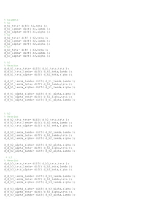
44. d_d_h3_teta_lamda_0= 0;
d_d_h3_teta_alpha_0= 0;
d_d_h3_lamda_lamda_0= 0;
d_d_h3_lamda_teta_0= 0;
d_d_h3_lamda_alpha_0= 0;
d_d_h3_alpha_alpha_0= -467*sin(alpha + 279/100);
d_d_h3_alpha_teta_0= 0;
d_d_h3_alpha_lamda_0= 0;
%%%%%%%%%%%%%%%%%%%% Stiffness matrix
Stiffness_jacobian= [ d_a_teta_0, d_a_lamda_0, d_a_alpha_0;
d_j_teta_0, d_j_lamda_0, d_j_alpha_0;
d_h_teta_0, d_h_lamda_0, d_h_alpha_0 ];
kf_vector= [ k1,k2,k3 ]; % vector of the actuator stiffnesses
Kf=diag( kf_vector );
K_el_I_1= Stiffness_jacobian'*Kf*Stiffness_jacobian;
Stiffness_hessian_1= [ d_d_a_teta_teta_0, d_d_a_teta_lamda_0, d_d_a_teta_alpha_0
d_d_a_lamda_teta_0, d_d_a_lamda_lamda_0, d_d_a_lamda_alpha_0
d_d_a_alpha_teta_0, d_d_a_alpha_lamda_0, d_d_a_alpha_alpha_0
];
Stiffness_hessian_2= [ d_d_j_teta_teta_0, d_d_j_teta_lamda_0, d_d_j_teta_alpha_0
d_d_j_lamda_teta_0, d_d_j_lamda_lamda_0, d_d_j_lamda_alpha_0
d_d_j_alpha_teta_0, d_d_j_alpha_lamda_0, d_d_j_alpha_alpha_0
];
Stiffness_hessian_3= [ d_d_h_teta_teta_0, d_d_h_teta_lamda_0, d_d_h_teta_alpha_0
d_d_h_lamda_teta_0, d_d_h_lamda_lamda_0, d_d_h_lamda_alpha_0
d_d_h_alpha_teta_0, d_d_h_alpha_lamda_0, d_d_h_alpha_alpha_0
];
delta_1_static= 51.27;
delta_2_static= 0.71;
delta_3_static= 31.81;
K_el_I_1I_1= k1*delta_1_static*Stiffness_hessian_1 +
k2*delta_2_static*Stiffness_hessian_2 + k3*delta_3_static*Stiffness_hessian_3;
Height_hessian_1= [ d_d_h1_teta_teta_0, d_d_h1_teta_lamda_0, d_d_h1_teta_alpha_0
d_d_h1_lamda_teta_0, d_d_h1_lamda_lamda_0, d_d_h1_lamda_alpha_0

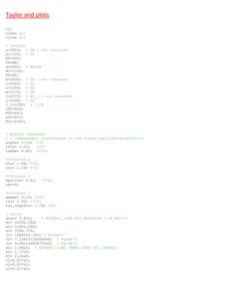
45. d_d_h1_alpha_teta_0, d_d_h1_alpha_lamda_0, d_d_h1_alpha_alpha_0
];
Height_hessian_2= [ d_d_h2_teta_teta_0, d_d_h2_teta_lamda_0, d_d_h2_teta_alpha_0
d_d_h2_lamda_teta_0, d_d_h2_lamda_lamda_0, d_d_h2_lamda_alpha_0
d_d_h2_alpha_teta_0, d_d_h2_alpha_lamda_0, d_d_h2_alpha_alpha_0
];
Height_hessian_3= [ d_d_h3_teta_teta_0, d_d_h3_teta_lamda_0, d_d_h3_teta_alpha_0
d_d_h3_lamda_teta_0, d_d_h3_lamda_lamda_0, d_d_h3_lamda_alpha_0
d_d_h3_alpha_teta_0, d_d_h3_alpha_lamda_0, d_d_h3_alpha_alpha_0
];
K_g= grav* ( m1*Height_hessian_1 + m2*Height_hessian_2 + m3*Height_hessian_3 );
K= K_el_I_1 + K_el_I_1I_1 + K_g;
%%%%%%%%%%%%%%%%%%%% Damping matrix
Rf_vector= [ c1,c2,c3 ];
Rf= diag( Rf_vector );
R= Stiffness_jacobian'*Rf*Stiffness_jacobian;
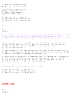
syms teta_dot lamda_dot alpha_dot F0_ext de_alpha de_lamda de_teta
v1x= -teta_dot*LG1*cos(6.81-teta)-alpha_dot*NC*cos(alpha)-lamda_dot*n*sin(lamda);
v1y= teta_dot*LG1*sin(6.81-teta)-alpha_dot*NC*sin(alpha)+lamda_dot*n*cos(lamda);
%%%%%%% Mass Jacobian Jm
Jm_vector= [ m1,m1,m2,m3,J1,J2,J3 ];
Mf= diag( Jm_vector );
Jm= [ -LG1*cos(6.81-teta), -NC*cos(alpha), -n*sin(lamda)
LG1*sin(6.81-teta), -NC*sin(alpha), n*cos(lamda)
0, 0, CG2
0, 0, FG3
1, 0, 0
0, 0, 1
0, 0, 1 ];
M= Jm'*Mf*Jm;

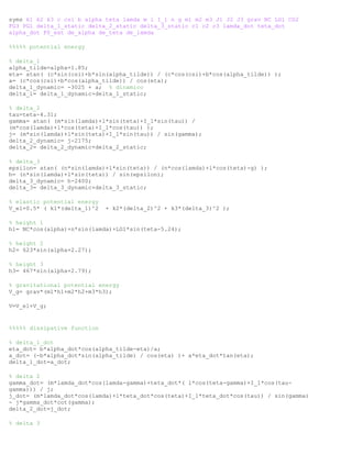
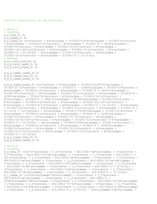
46. %%%%%% Virtual work linearization / Force jacobian
de_s_x= -NC*cos(alpha)*de_alpha - n*sin(lamda)*de_lamda - ( LG1*sin(teta-5.24) +
PG1*sin(6.14-teta) )*de_teta;
de_s_y= -NC*sin(alpha)*de_alpha - n*cos(lamda)*de_lamda + ( LG1*cos(teta-5.24) -
PG1*cos(6.14-teta) )*de_teta;
Jf= [ -LG1*sin(teta-5.24) - PG1*sin(6.14-teta), - n*sin(lamda), -NC*cos(alpha)
LG1*cos(teta-5.24) - PG1*cos(6.14-teta), - n*cos(lamda), -NC*sin(alpha)
];
force_vector= [ F0_ext*cosd(15); -F0_ext*sind(15) ];
Q= Jf'*force_vector;
%%
%%%%%%%%%%% Natural frequencies and vibration modes
M= 1.0e+11 *[ 0.1485 -0.0479 -0.3974
-0.0479 0.3944 -0.3723
-0.3974 -0.3723 1.9553 ];
K= 1.0e+12 * [ 1.6607 -0.2285 0
-0.2285 0.2390 0
0 0 0.2513 ];
R= 1.0e+10* [ 1.6630 -0.2309 0
-0.2309 0.2392 0
0 0 0.2496 ];
A= inv(M)*K;
[ phi,natural_frequencies_squared ]= eig(A);
natural_frequencies= sqrt(natural_frequencies_squared);
%%%%%%%%%%% FRF frequency response function
F0_ext=1;
LG1=675;
alpha= 1.19; %68
teta= 6.23; %357
lamda= 4.80; %275;
PG1=2550;
n=2300;
NC=1100;
force_vector= [ F0_ext*cosd(15); -F0_ext*sind(15) ];
Jf= [ -LG1*sin(teta-5.24) - PG1*sin(6.14-teta), - n*sin(lamda), -NC*cos(alpha)
LG1*cos(teta-5.24) - PG1*cos(6.14-teta), - n*cos(lamda), -NC*sin(alpha)
];
Q= Jf'*force_vector;
max_natural_frequency=max(max(natural_frequencies));
omega=linspace(0,2*max_natural_frequency,300); % grafico fino a tre volte la
massima frequenza
length_omega=length(omega);
TETA=[];
LAMDA=[];

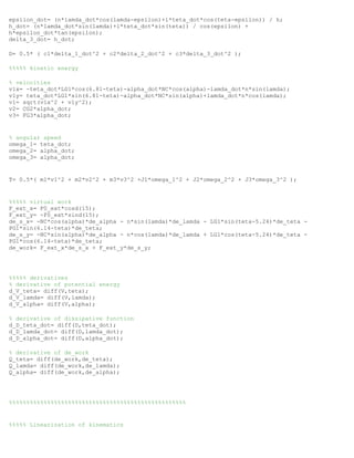
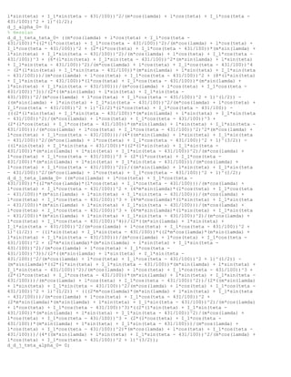
47. ALPHA=[];
for ii=1:length_omega
AA= -(omega(ii))^2*M + 1i*omega(ii)*R + K;
z_0= inv(AA)*Q;
teta_0= z_0(1);
lamda_0= z_0(2);
alpha_0= z_0(3);
TETA= [ TETA,teta_0 ];
LAMDA= [ LAMDA,lamda_0 ];
ALPHA= [ ALPHA,alpha_0 ];
end
amplitude_TETA= abs( TETA );
amplitude_LAMDA= abs( LAMDA );
amplitude_ALPHA= abs( ALPHA );
angle_TETA= angle( TETA );
angle_LAMDA= angle( LAMDA );
angle_ALPHA= angle( ALPHA );
figure(1)
plot( omega,amplitude_TETA )
title( 'amplitude teta' )
xlabel('Omega')
ylabel('FRF theta')
figure(2)
plot( omega,amplitude_LAMDA )
title( 'amplitude lamda' )
xlabel('Omega')
ylabel('FRF lambda')
figure(3)
plot( omega,amplitude_ALPHA )
title( 'amplitude alpha' )
xlabel('Omega')
ylabel('FRF alpha')
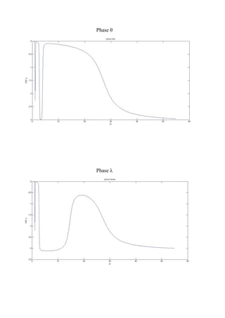
figure(4)
plot( omega,angle_TETA )
title( 'phase teta' )
xlabel('Omega')
ylabel('FRF theta')
figure(5)
plot( omega,angle_LAMDA )
title( 'phase lamda' )
xlabel('Omega')
ylabel('FRF lambda')
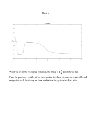
figure(6)
plot( omega,angle_ALPHA )
title( 'phase alpha' )
xlabel('Omega')
ylabel('FRF alpha')