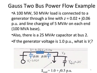
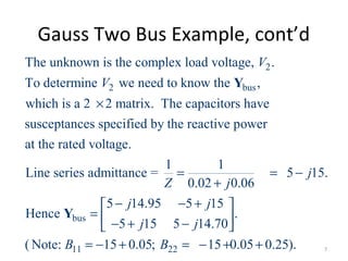
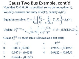
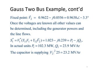
This document discusses a lecture on power flow analysis in a power systems engineering course. It provides announcements about homework assignments and an upcoming midterm exam. It also discusses examples of the Gauss two bus power flow method and the inclusion of PV generator buses in the Gauss-Seidel iteration method. Key concepts covered include slack buses, generator reactive power limits, and methods to accelerate Gauss-Seidel convergence.

1. EE 369
POWER SYSTEM ANALYSIS
Lecture 11
Power Flow
Tom Overbye and Ross Baldick
1

2. Announcements
• Start reading Chapter 6 for lectures 11 and 12.
• Homework 8 is 3.1, 3.3, 3.4, 3.7, 3.8, 3.9, 3.10,
3.12, 3.13, 3.14, 3.16, 3.18; due 10/29.
• Homework 9 is 3.20, 3.23, 3.25, 3.27, 3.28,
3.29, 3.35, 3.38, 3.39, 3.41, 3.44, 3.47; due
11/5.
• Midterm 2, Thursday, November 12, covering
up to and including material in HW9.
2

3. Wind Blade Failure
Photo source: Peoria Journal Star
Several years ago, a 140 foot,
6.5 ton blade broke off from a
Suzlon Energy wind turbine.
The wind turbine is located
in Illinois. Suzlon Energy is
one of the world’s largest
wind turbine manufacturers;
its shares fell 39% following
the accident. No one was hurt
and wind turbines failures
are extremely rare events.
(Vestas and Siemens turbines
have also failed.) 3

4. Thermal Plants Can Fail As Well: Another Illinois
Failure, Fall 2007
4

5. Springfield, Illinois City Water,
Light and Power Explosion, Fall
2007
5

6. Gauss Two Bus Power Flow Example
•A 100 MW, 50 MVAr load is connected to a
generator through a line with z = 0.02 + j0.06
p.u. and line charging of 5 MVAr on each end
(100 MVA base).
•Also, there is a 25 MVAr capacitor at bus 2.
•If the generator voltage is 1.0 p.u., what is V2?
SLoad = 1.0 + j0.5 p.u. 6
j0.05 j0.05

7. Gauss Two Bus Example, cont’d
2
2 bus
The unknown is the complex load voltage, .
To determine we need to know the ,
which is a 2 2 matrix. The capacitors have
susceptances specified by the reactive power
at the rated voltage.
Line
V
V
×
Y
bus
11 22
1 1
series admittance = 5 15.
0.02 0.06
5 14.95 5 15
Hence .
5 15 5 14.70
( Note: 15 0.05; 15 0.05 0.25).
j
Z j
j j
j j
B B
= = −
+
− − + 
=  − + − 
= − + = − + +
Y
7

8. Gauss Two Bus Example, cont’d
1 1
2
*
2
2 2 2*
22 1, 22
( 1)
2
2
Note that =1.0 0 is specified, so we do not update .
We only consider one entry of ( ), namely ( ).
1 S
Equation to solve: ( ).
1 1 0.5
Update:
5 14.70 (
n
k k
k k
V V
h V h V
V Y V h V
Y V
j
V
j V
ν
= ≠
+
∠
 
= − = ÷
 
− +
=
−
∑
( )
(0)
2
( ) ( )
2 2
( 5 15)(1.0 0)
)*
Guess 1.0 0 (this is known as a flat start)
0 1.000 0.000 3 0.9622 0.0556
1 0.9671 0.0568 4 0.9622 0.0556
2 0.9624 0.0553
v v
j
V
v V v V
j j
j j
j
ν
 
− − + ∠ ÷
 
= ∠
+ −
− −
− 8

9. Gauss Two Bus Example, cont’d
2
* *
1 1 11 1 12 2 1 1
ˆFixed point: 0.9622 0.0556 0.9638 3.3
Once the voltages are known all other values can
be determined, including the generator powers and
the line flows.
ˆ( ) 1.023 0.239 ,
V j
S V Y V Y V j P jQ
= − = ∠ − °
= + = − = −
1 1
2
2
In actual units 102.3 MW, 23.9 MVAr
The capacitor is supplying 25 23.2 MVAr
P Q
V
= =
=
9

10. Slack Bus
In previous example we specified S2 and V1
and then solved for S1 and V2.
We can not arbitrarily specify S at all buses
because total generation must equal total
load + total losses.
We also need an angle reference bus.
To solve these problems we define one bus
as the “slack” bus. This bus has a fixed
voltage magnitude and angle, and a varying
real/reactive power injection. In the
previous example, this was bus 1. 10

11. Gauss for Systems with Many Buses
*
( 1) ( )
( )*
1,
( ) ( ) ( )
1 2
( 1)
With multiple bus systems we could calculate
new values of the voltages as follows:
S1
( , ,..., )
But after we've determined , it is
i
i
n
v vi
i ik kv
ii k k i
v v v
i n
v
i
V
V Y V
Y V
h V V V
V
+
= ≠
+
 
= − ÷
 ÷
 
=
∑
( )
a better estimate
of the voltage at bus than , so it makes sense to use
this new value. Using the latest values is known as the
Gauss-Seidel iteration.
v
ii V
11

12. Gauss-Seidel Iteration
( 1) ( ) ( ) ( )
2 12 2 3
( 1) ( 1) ( ) ( )
3 13 2 3
( 1) ( 1) ( 1) ( ) ( )
4 14 2 3 4
( 1) ( 1) (
1 2 3
Immediately use the new voltage estimates:
( , , , , ) (bus 1 is slack),
( , , , , )
( , , , , )
( , ,
v v v v
n
v v v v
n
v v v v v
n
v v v
n n
V h V V V V
V h V V V V
V h V V V V V
V h V V V
+
+ +
+ + +
+ +
= …
= …
= …
=
M
1) ( 1) ( )
4, , )
Gauss-Seidel usually works better than the Gauss, and
is actually easier to implement.
Gauss-Seidel is used in practice instead of Gauss.
v v
nV V+ +
…
12

13. Three Types of Power Flow Buses
There are three main types of buses:
– Load (PQ), at which P and Q are fixed; goal is to
solve for unknown voltage magnitude and angle at
the bus.
– Slack at which the voltage magnitude and angle
are fixed; iteration solves for unknown P and Q
injections at the slack bus
– Generator (PV) at which P and |V| are fixed;
iteration solves for unknown voltage angle and Q
injection at bus:
special coding is needed to include PV buses in the
Gauss-Seidel iteration. 13

14. Inclusion of PV Buses in G-S
* *
1
( ) ( )* ( )
1
To solve for at a PV bus we must first make a
guess of using the power flow equation:
Hence Im is an
estimate of the reactive power injectio
k
i
i
n
i i ik k i i
k
n
v v v
i i ik
k
V
Q
S V Y V P jQ
Q V Y V
=
=
= = −
 
= −  
 
∑
∑
( ) ( )
n.
For the Gauss iteration we use the known value
of real power and the estimate of the reactive power:
v v
i i iS P jQ= + 14

15. Inclusion of PV Buses, cont'd
( 1)
( )*
( 1) ( )
( )*
1,
( 1) ( 1)
( 1)
( 1)
Tentatively solve for
1
In update, set .
But since is specified, replace by .
That is, set
i
v
i
v n
v vi
i ik kv
ii k k i
v
i i
v
i i i
i i
V
S
V Y V
Y V
V V
V V V
V V
ν
ν
+
+
= ≠
+ +
+
+
 
= − ÷
 ÷
 
∠ = ∠
=
∑%
%
%
15

16. Two Bus PV Example
Bus 1
(slack bus)
Bus 2
V1 = 1.0 V2 = 1.05
P2 = 0 MW
z = 0 .0 2 + j 0 .0 6
Consider the same two bus system from the previous
example, except the load is replaced by a generator
16
j0.05j0.05

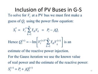
17. Two Bus PV Example, cont'd
( ) ( )* ( )
22 2
1
( ) ( )* ( ) ( )*
21 221 2 2 2
( )* ( )*
( 1) ( ) ( )2 2
2 212 1( )* ( )*
22 221, 22 2
(0)
2
( ) ( 1) ( 1)
2 2 2
Im ,
Im[ ]
1 1
Guess 1.05 0
0 0 0.457
k
n
v v
k
k
n
k k
k k
v v v
Q V Y V
Y V V Y V V
S S
V Y V Y V
Y YV V
V
v S V V
j
ν
ν ν ν ν
ν ν
ν ν ν
ν ν
=
+
= ≠
+ +
 
= −  
 
= − +
   
= − = − ÷  ÷
  
= ∠ °
+
∑
∑%
%
1.045 0.83 1.050 0.83
1 0 0.535 1.049 0.93 1.050 0.93
2 0 0.545 1.050 0.96 1.050 0.96
j
j
∠ − ° ∠ − °
+ ∠ − ° ∠ − °
+ ∠ − ° ∠ − ° 17

18. Generator Reactive Power Limits
The reactive power output of generators
varies to maintain the terminal voltage; on
a real generator this is done by the exciter.
To maintain higher voltages requires more
reactive power.
Generators have reactive power limits,
which are dependent upon the generator's
MW output.
These limits must be considered during the
power flow solution. 18

19. Generator Reactive Limits, cont'd
During power flow once a solution is
obtained, need to check if the generator
reactive power output is within its limits
If the reactive power is outside of the limits,
then fix Q at the max or min value, and re-
solve treating the generator as a PQ bus
– this is know as "type-switching"
– also need to check if a PQ generator can again
regulate
Rule of thumb: to raise system voltage we
need to supply more VArs. 19

20. Accelerated G-S Convergence
( 1) ( )
( 1) ( ) ( ) ( )
(
Previously in the Gauss-Seidel method we were
calculating each value as
( )
To accelerate convergence we can rewrite this as
( )
Now introduce "acceleration parameter"
v v
v v v v
x
x h x
x x h x x
x
α
+
+
=
= + −
1) ( ) ( ) ( )
( ( ) )
With = 1 this is identical to standard Gauss-Seidel.
Larger values of may result in faster convergence.
v v v v
x h x xα
α
α
+
= + −
20

21. Accelerated Convergence, cont’d
( 1) ( ) ( ) ( )
Consider the previous example: 1 0
(1 )
Matlab code: alpha=1.2;x=x0;x=x+alpha*(1+sqrt(x)-x).
Comparison of results with different values of
1 1.2 1.5 2
0 1 1 1 1
1 2 2.20 2.5 3
2
v v v v
x x
x x x xα
α
ν α α α α
+
− − =
= + + −
= = = =
2.4142 2.5399 2.6217 2.464
3 2.5554 2.6045 2.6179 2.675
4 2.5981 2.6157 2.6180 2.596
5 2.6118 2.6176 2.6180 2.626 21

22. Gauss-Seidel Advantages
Each iteration is relatively fast (computational
order is proportional to number of branches +
number of buses in the system).
Relatively easy to program.
22

23. Gauss-Seidel Disadvantages
Tends to converge relatively slowly, although
this can be improved with acceleration.
Has tendency to fail to find solutions,
particularly on large systems.
Tends to diverge on cases with negative
branch reactances (common with
compensated lines)
Need to program using complex numbers.
23

24. Newton-Raphson Algorithm
The second major power flow solution
method is the Newton-Raphson algorithm
Key idea behind Newton-Raphson is to use
sequential linearization
General form of problem: Find an such that
( ) 0
x
f x =
24

25. Newton-Raphson Method (scalar)
( )
( )
( )
( ) ( ) ( ) ( ) ( )
2 2( ) ( )
2
1. Represent by a Taylor series about the
current guess . Write for the deviation
from :
( ) ( ) ( )
1
( )
2
higher order terms.
v v v v v
v v
f
x x
x
df
f x x f x x x
dx
d f
x x
dx
ν
ν
∆
 + ∆ = + ∆ +
  
 
+ ∆ + 
 
25

26. Newton-Raphson Method, cont’d
( ) ( ) ( ) ( ) ( )
( )
1
( ) ( ) ( )
2. Approximate by neglecting all terms
except the first two
( ) ( ) ( )
3. Set linear approximation equal to zero
and solve for
( ) ( )
4. Sol
v v v
v
v v v
f
df
f x x f x x x
dx
x
df
x x f x
dx
ν ν
−
 + ∆ ≈ + ∆
  
∆
 ∆ = −
  
( 1) ( ) ( )
ve for a new estimate of solution:
v v v
x x x+
= + ∆ 26

27. Newton-Raphson Example
2
1
( ) ( ) ( )
( ) ( ) 2
( )
( 1) ( ) ( )
( 1) ( ) ( ) 2
( )
Use Newton-Raphson to solve ( ) 0,
where: ( )= 2.
The iterative update is:
( ) ( )
1
(( ) 2)
2
1
(( ) 2).
2
v v v
v v
v
v v v
v v v
v
f x
f x x
df
x x f x
dx
x x
x
x x x
x x x
x
−
+
+
=
−
 ∆ = −
  
 ∆ = − −
  
= + ∆
 = − −
   27

28. Newton-Raphson Example, cont’d
( 1) ( ) ( ) 2
( )
(0)
( ) ( ) ( )
3 3
6
1
(( ) 2)
2
Matlab code: x=x0; x = x-(1/(2*x))*(x^2-2).
Guess 1. Iteratiting, we get:
( )
0 1 1 0.5
1 1.5 0.25 0.08333
2 1.41667 6.953 10 2.454 10
3 1.41422 6.024 10
v v v
v
v v v
x x x
x
x
x f x xν
+
− −
−
 = − −
  
=
∆
−
−
× − ×
×
28

29. Sequential Linear Approximations
Function is f(x) = x2
- 2.
Solutions to f(x) = 0 are points where
f(x) intersects x axis.
At each
iteration the
N-R method
uses a linear
approximation
to determine
the next value
for x
29

30. Newton-Raphson Comments
• When close to the solution the error
decreases quite quickly -- method has what is
known as “quadratic” convergence:
– number of correct significant figures roughly
doubles at each iteration.
• f(x(v)
) is known as the “mismatch,” which we
would like to drive to zero.
• Stopping criteria is when f(x(v)
)  < ε
30

31. Newton-Raphson Comments
• Results are dependent upon the initial guess.
What if we had guessed x(0)
= 0, or x(0)
= -1?
• A solution’s region of attraction (ROA) is the
set of initial guesses that converge to the
particular solution.
• The ROA is often hard to determine.
31

32. Multi-Variable Newton-Raphson
1 1
2 2
Next we generalize to the case where is an -
dimension vector, and ( ) is an -dimensional
vector function:
( )
( )
( )
( )
Again we seek a solution of ( ) 0.
n n
n
n
x f
x f
x f
   
   
   = =
   
   
   
=
x
f x
x
x
x f x
x
f x
M M
32

33. Multi-Variable Case, cont’d
i
1 1
1 1 1 2
1 2
1
1 2
1 2
The Taylor series expansion is written for each f ( )
( ) ( ) ( ) ( )
( ) higher order terms
( ) ( ) ( ) ( )
( ) higher order terms
n
n
n n
n n
n
n
n
f f
f x x f x x x x x
x x
f
x x
x
f f
f x x f x x x x x
x x
f
x x
x
∂ ∂
+ ∆ = + ∆ + ∆ +…
∂ ∂
∂
∆ +
∂
∂ ∂
+ ∆ = + ∆ + ∆ +…
∂ ∂
∂
∆ +
∂
x
M
33

34. Multi-Variable Case, cont’d
1 1 1
1 2
1 1
2 2 2
2 2
1 2
1 2
This can be written more compactly in matrix form
( ) ( ) ( )
( )
( ) ( ) ( )( )
( )
( )
( ) ( ) ( )
n
n
n
n n n
n
f f f
x x x
f x
f f f
f x
x x x
f
f f f
x x x
∂ ∂ ∂ 
 ∂ ∂ ∂
∆  
∂ ∂ ∂   ∆
   ∂ ∂ ∂= +
  
  
   ∂ ∂ ∂
 
∂ ∂ ∂ 
x x x
x
x x xx
f x +Δx
x
x x x
L
L
M
M O O M
L
higher order terms
nx
 
 
 
 
 ∆ 
+
M
34

35. Jacobian Matrix
1 1 1
1 2
2 2 2
1 2
1 2
The by matrix of partial derivatives is known
as the Jacobian matrix, ( )
( ) ( ) ( )
( ) ( ) ( )
( )
( ) ( ) ( )
n
n
n n n
n
n n
f f f
x x x
f f f
x x x
f f f
x x x
∂ ∂ ∂ 
 ∂ ∂ ∂
 
∂ ∂ ∂ 
 ∂ ∂ ∂=
 
 
 ∂ ∂ ∂
 
∂ ∂ ∂  
J x
x x x
x x x
J x
x x x
L
L
M O O M
L
35

36. Multi-Variable N-R Procedure
Derivation of N-R method is similar to the scalar case
( ) ( ) ( ) higher order terms
( ) ( ) ( )
To seek solution to ( ) 0, set linear
approximation equal to zero: 0 ( ) ( ) .
+ ∆ = + ∆ +
+ ∆ ≈ + ∆
+ ∆ =
= + ∆
∆ = −
f x x f x J x x
f x x f x J x x
f x x
f x J x x
x 1
( 1) ( ) ( )
( 1) ( ) ( ) 1 ( )
( )
( ) ( )
( ) ( )
Iterate until ( )
v v v
v v v v
v
ε
−
+
+ −
= + ∆
= −
<
J x f x
x x x
x x J x f x
f x
36

37. Multi-Variable Example
1
2
2 2
1 1 2
2 2
2 1 2 1 2
1 1
1 2
2 2
1 2
Solve for = such that ( ) 0 where
( ) 2 8
( ) 4
First symbolically determine the Jacobian
( ) ( )
( ) =
( ) ( )
x
x
f x x x
f x x x x x
f f
x x
x x
f f
x x
x x
 
= 
 
= + −
= − + −
∂ ∂ 
 ∂ ∂
 
∂ ∂ 
 ∂ ∂ 
x f x
J x
37

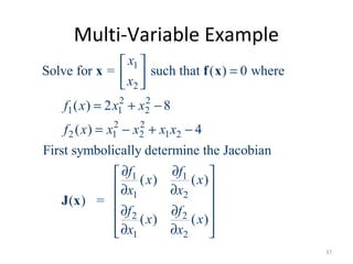
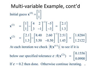
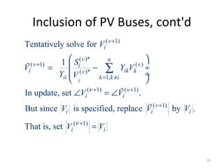
38. Multi-variable Example, cont’d
1 2
1 2 1 2
1
1 1 2 1
2 1 2 1 2 2
4 2
( ) =
2 2
4 2 ( )
Then
2 2 ( )
Matlab code: x1=x10; x2=x20;
f1=2*x1^2+x2^2-8;
f2=x1^2-x2^2+x1*x2-4;
J = [4*x1 2*x2; 2*x1+x2 x1-2*x2];
[x1;x2] =
x x
x x x x
x x x f
x x x x x f
−
 
 + − 
∆     
= −     ∆ + −     
J x
x
x
[x1;x2]-inv(J)*[f1;f2].
38

39. Multi-variable Example, cont’d
(0)
1
(1)
1
(2)
( )
1
Initial guess
1
1 4 2 5 2.1
1 3 1 3 1.3
2.1 8.40 2.60 2.51 1.8284
1.3 5.50 0.50 1.45 1.2122
At each iteration we check ( ) to see if itν
−
−
 
=  
 
−       
= − =       − −       
       
= − =       −       
x
x
x
f x
(2)
is
0.1556
below our specified tolerance : ( )
0.0900
If = 0.2 then done. Otherwise continue iterating.
ε
ε
 
=  
 
f x
39