This document describes using the Gauss-Seidel method to solve non-linear load flow equations in MATLAB. The objective is to develop a program that models power flow through a system using an iterative Gauss-Seidel algorithm. It provides the theory behind load flow analysis and outlines the Gauss-Seidel method. The problem statement gives sample system data and instructions to find the voltages and angles at three buses after the first iteration.

1. EXPERIMENT-4
OBJECTIVE
To develop a computer program to solve the set of non linear load flow equations using
Gauss seidal load flow algorithm.
SOFTWARE USED
MATLAB
THEORY
Load flow analysis is the most frequently performed system study by electric utilities. This
analysis is performed on a symmetrical steady-state operating condition of a power system
under ‘normal’ mode of operation and aims at obtaining bus voltages and line/transformer
flows for a given load condition. This information is essential both for long term planning
and next day operational planning. In long term planning, load flow analysis helps in
investigating the effectiveness of alternative plans and choosing the ‘best’ plan for system
expansion to meet the projected operating state. In operational planning, it helps in choosing
the ‘best’ unit commitment plan and generation schedules to run the system efficiently for
them next day’s load condition without violating the bus voltage and line flow operating
limits.
The Gauss seidal method is an iterative algorithm for solving a set of non- linear algebraic
equations. The relationship between network bus voltages and currents may be represented
by either loop equations or node equations. Node equations are normally preferred because
the number of independent node equation is smaller than the number of independent loop
equations.
The network equations in terms of the bus admittance matrix can be written as,
퐼bus=[Ybus]푉bus (1)
For a n bus system, the above performance equation can be expanded as,
[
퐼1
퐼2
⋮
⋮
퐼푝
⋮
퐼푛]
=
푌11 푌12 … 푌1푝 푌1푛
푌12 푌22 … 푌2푝 푌2푛
⋮ ⋮ ⋮ ⋮
⋮ ⋮ ⋮ ⋮
푌푝1 푌푝2 … 푌푝푝 푌푝푛
⋮ ⋮ ⋮ ⋮
푌푛1 푌푛2 … 푌푛푝 푌푛푛
[
]
푉1
푉2
⋮
⋮
푉푝
⋮
푉푛]
[
(2)
where n is the total number of nodes.
Vp is the phasor voltage to ground at node p.
Ip is the phasor current flowing into the network at node p.

2. At the pth bus, current injection:
퐼푝=Yp1V1+ Yp2V2+YppVp+…….YpnVn
푛푞
= Σ 푌푝푞 푉푞
푛
푞=1
푞≠푝
=1 = 푌푝푝푉푝 + Σ 푌푝푞 푉푞
(3)
Vp = 1
Ypp
[퐼푝 −
푛
푞=1
푞≠푝
Σ 푌푝푞 푉푞
] (4)
At bus p , we can write Pp –jQp=Vp*Ip
Hence, the current at any node p is related to P, Q and V as follows:
∴ Ip =
(Pp−jQp )
Vp ∗
(for any bus p except slack bus s)
Substituting for Ip in Equation (4),
Vp =
1
Ypp
[
(Pp − jQp )
∗ − Σ 푌푝푞 푉푞
Vp
푛
푞=1
푞≠푝
]
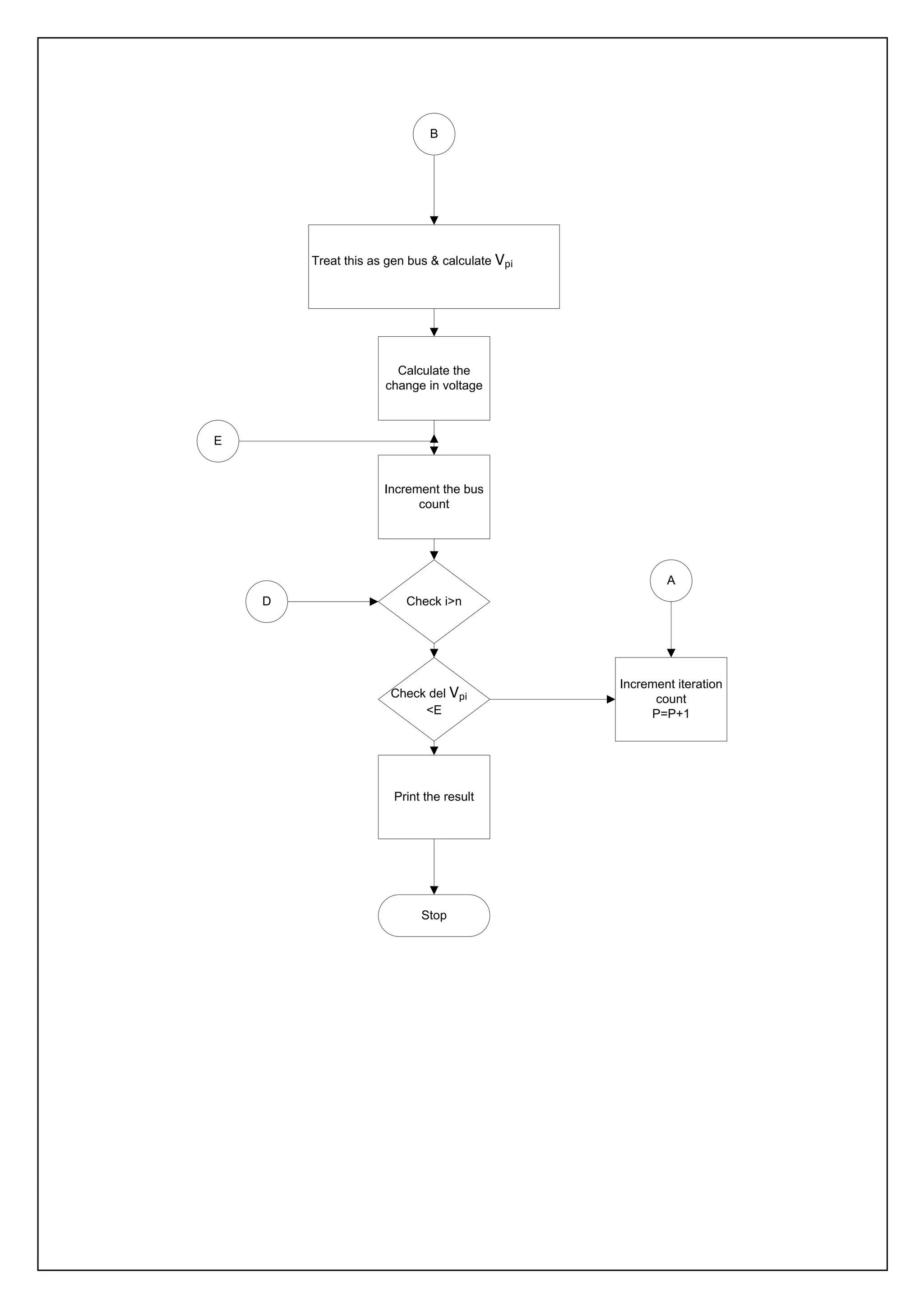
ALGORITHM:
Step 1: Read the input data.
Step 2: Find out the admittance matrix.
Step 3: Choose the flat voltage profile 1+j0 to all buses except slack bus.
Step 4: Set the iteration count p = 0 and bus count i = 1.
Step 5: Check the slack bus, if it is the generator bus then go to the next step otherwise go to
Next step 7.
Step 6: Before the check for the slack bus if it is slack bus then go to step 11 otherwise go to
Next step.
Step 7: Check the reactive power of the generator bus within the given limit.
Step 8: If the reactive power violates a limit then treat the bus as load bus.
Step 9: Calculate the phase of the bus voltage on load bus
Step 10: Calculate the change in bus voltage of the repeat step mentioned above until all the
bus voltages are calculated.
Step 11: Stop the program and print the results
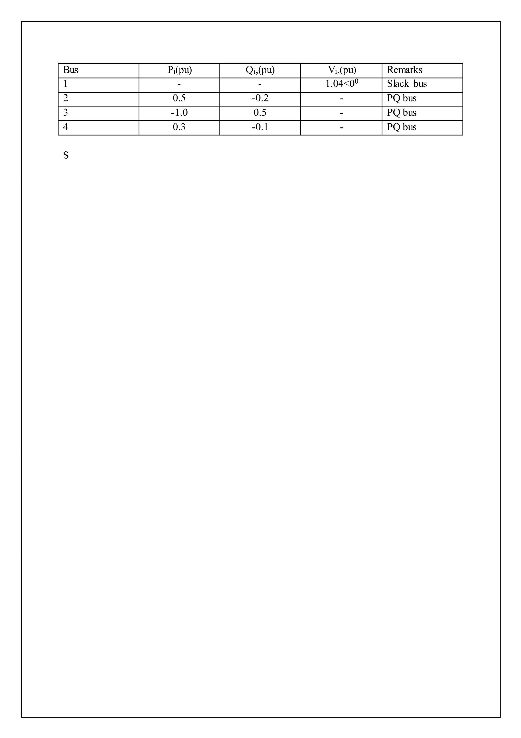
PROBLEM STATEMENT
For the sample system the generators are connected at all the four buses by loads are at buses
2 and 3. Values of real and reactive power are listed in tables.All buses other than the slack
are PQ type.
Assuming a flat voltage start find the voltages and bus angles at the three buses at the end of
the first GS iteration

3. Bus Pi(pu) Qi,(pu) Vi,(pu) Remarks
1 - - 1.04<00 Slack bus
2 0.5 -0.2 - PQ bus
3 -1.0 0.5 - PQ bus
4 0.3 -0.1 - PQ bus
S

4. Treat this as gen bus & calculate Vpi
Calculate the
change in voltage
Increment the bus
count
Check i>n
Check del Vpi
<E
Increment iteration
count
P=P+1
Print the result
Stop
D
A
E
B