Download as PDF, PPTX


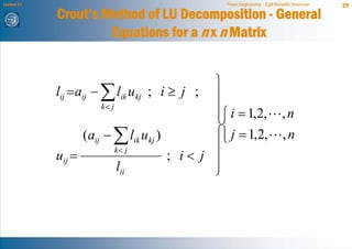
![Lecture 21 Power Engineering - Egill Benedikt Hreinsson 25
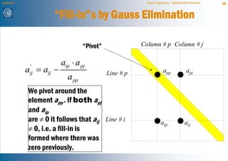
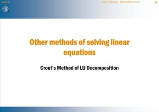
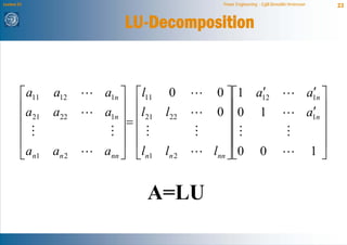
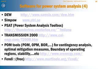
An Example of Crout’s Method of LU Decomposition
(4x4) (2)
⎡ a11 a12 a13 a14 ⎤ ⎡l11 0 0 0 ⎤⎡1 u12 u13 u14 ⎤
⎢a a22 a23 a24 ⎥ ⎢l21 l22 0 0 ⎥ ⎢0 1 u23 u24 ⎥
⎢ 21 ⎥= ⎢ ⎥⎢ ⎥
⎢ a31 a32 a33 a34 ⎥ ⎢l31 l32 l33 0 ⎥ ⎢0 0 1 u34 ⎥
⎢ ⎥ ⎢ ⎥⎢ ⎥
⎣a41 a42 a43 a44 ⎦ ⎣l41 l42 l43 l44 ⎦⎣0 0 0 1⎦
a21 =l21 ⇒ l21 =a21
2nd row of the L a22 =l21u12 +l22 ⇒ l22 =a22 −l21u12
and U matrices [a23 −l21u13 ]
on the right side: a23 =l21u13 +l22 u23 ⇒ u23 =
l22
a24 =l21u14 +l22 u24 ⇒ u24 =
[a24 −l21u14 ]
l22](https://image.slidesharecdn.com/rk21powerflowsparse2-130205204327-phpapp02/85/Rk21-power-flow_sparse2-25-320.jpg)
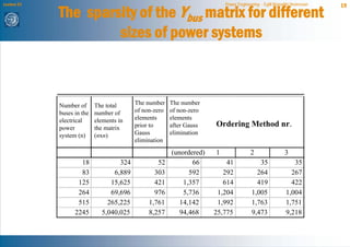
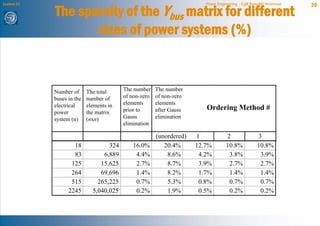
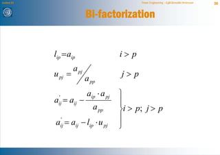
![Lecture 21 Power Engineering - Egill Benedikt Hreinsson 26
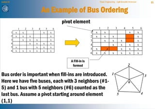
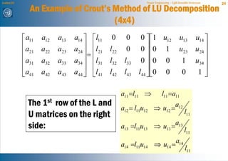
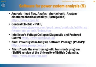
An Example of Crout’s Method of LU Decomposition (4x4)
(3)
⎡ a11 a12 a13 a14 ⎤ ⎡l11 0 0 0 ⎤⎡1 u12 u13 u14 ⎤
⎢a a22 a23 a24 ⎥ ⎢l21 l22 0 0 ⎥ ⎢0 1 u23 u24 ⎥
⎢ 21 ⎥= ⎢ ⎥⎢ ⎥
⎢ a31 a32 a33 a34 ⎥ ⎢l31 l32 l33 0 ⎥⎢0 0 1 u34 ⎥
⎢ ⎥ ⎢ ⎥⎢ ⎥
⎣a41 a42 a43 a44 ⎦ ⎣l41 l42 l43 l44 ⎦⎣0 0 0 1⎦
The 3rd row of a31 = l31 ⇒ l31 =a31
the L and U a32 = l31u12 +l32 ⇒ l32 =a32 −l31u12
matrices on a33 = l31u13 +l32 u23 +l33 ⇒ l33 = a33 −l31u13 −l32 u23
the right side: a34 = l31u14 +l32 u24 +l33u34 ⇒ u34 = [a34 −l31u14 −l32 u24 ]
1
l33](https://image.slidesharecdn.com/rk21powerflowsparse2-130205204327-phpapp02/85/Rk21-power-flow_sparse2-26-320.jpg)
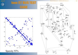
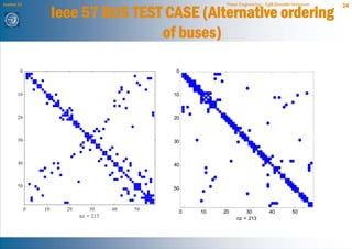


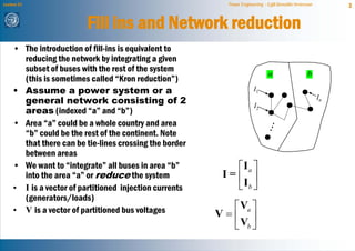
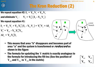
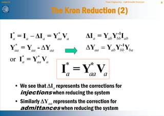
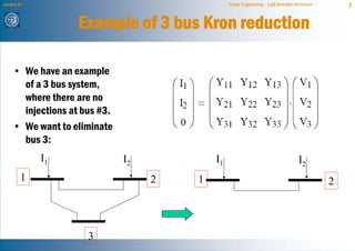
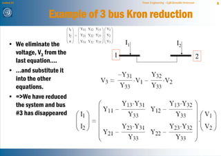
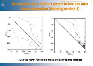
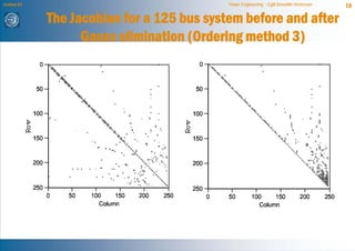
The document discusses network reduction techniques for solving power flow calculations more efficiently. It introduces the concept of "fill-ins" that occur during Gaussian elimination, which are analogous to introducing new branches when eliminating nodes during network reduction. The Kron reduction method is described, which eliminates nodes by integrating them into other areas of the network. This introduces corrections for injections and admittances in the reduced system, similar to fill-ins. An example of reducing a 3 bus system is provided. Different node ordering methods for Gaussian elimination are presented to minimize introduced fill-ins when solving large power networks.


![Ece4762011 lect11[1]](https://cdn.slidesharecdn.com/ss_thumbnails/ece4762011lect111-170908023044-thumbnail.jpg?width=640&height=640&fit=bounds)


