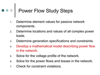
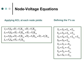
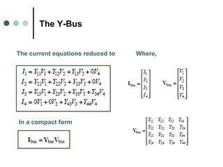
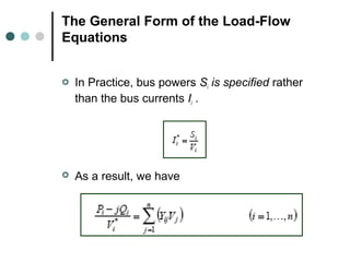
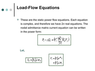
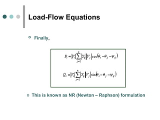
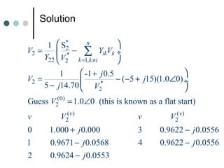
The document provides information about power flow analysis and solutions. It discusses how power flow analysis is fundamental to studying power systems and plays a key role in transmission planning. The document outlines the steps of a power flow study including developing the bus admittance matrix and node-voltage equations. It describes different bus types and how specifying certain values at each bus reduces the problem to solvable nonlinear equations. Iterative methods like Gauss-Seidel and Newton-Raphson are commonly used to solve the power flow equations.

1. EXPERT SYSTEMS AND SOLUTIONS
Email: expertsyssol@gmail.com
expertsyssol@yahoo.com
Cell: 9952749533
www.researchprojects.info
PAIYANOOR, OMR, CHENNAI
Call For Research Projects Final
year students of B.E in EEE, ECE,
EI, M.E (Power Systems), M.E
(Applied Electronics), M.E (Power
Electronics)
Ph.D Electrical and Electronics.
Students can assemble their hardware in our
Research labs. Experts will be guiding the
projects.

2. Power Flow Analysis
Well known as : Load Flow

3. The Power Flow Problem
 Power flow analysis is fundamental to the study of power
systems.
 In fact, power flow forms the core of power system analysis.
 power flow study plays a key role in the planning of additions
or expansions to transmission and generation facilities.
 A power flow solution is often the starting point for many other
types of power system analyses.
 In addition, power flow analysis is at the heart of contingency
analysis and the implementation of real-time monitoring
systems.

4. Problem Statement
For a given power network, with known complex
power loads and some set of specifications or
restrictions on power generations and voltages, solve
for any unknown bus voltages and unspecified
generation and finally for the complex power flow in the
network components.

5. Network Structure

6. Power Flow Study Steps
1. Determine element values for passive network
components.
2. Determine locations and values of all complex power
loads.
3. Determine generation specifications and constraints.
4. Develop a mathematical model describing power flow
in the network.
5. Solve for the voltage profile of the network.
6. Solve for the power flows and losses in the network.
7. Check for constraint violations.

7. Formulation of the Bus Admittance Matrix
 The first step in developing the mathematical model
describing the power flow in the network is the
formulation of the bus admittance matrix.
 The bus admittance matrix is an n*n matrix (where n is
the number of buses in the system) constructed from the
admittances of the equivalent circuit elements of the
segments making up the power system.
 Most system segments are represented by a combination
of shunt elements (connected between a bus and the
reference node) and series elements (connected
between two system buses).

8. Bus Admittance Matrix
Formulation of the bus admittance matrix follows two
simple rules:
1. The admittance of elements connected between node k
and reference is added to the (k, k) entry of the
admittance matrix.
2. The admittance of elements connected between nodes
j and k is added to the (j, j) and (k, k) entries of the
admittance matrix.
 The negative of the admittance is added to the (j, k) and
(k, j) entries of the admittance matrix.

9. Bus Admittance Matrix

10. Bus Admittance Matrix

11. Node-Voltage Equations
Applying KCL at each node yields: Defining the Y’s as

12. The Y-Bus
The current equations reduced to Where,
In a compact form

13. The General Form of the Load-Flow
Equations
 In Practice, bus powers Si is specified rather
than the bus currents Ii .
 As a result, we have

14. Load-Flow Equations
 These are the static power flow equations. Each equation
is complex, and therefore we have 2n real equations. The
nodal admittance matrix current equation can be written
in the power form:
Let,

15. Load-Flow Equations
 Finally,
o This is known as NR (Newton – Raphson) formulation

16. Gauss Power Flow
We first need to put the equation in the correct form
*
 n  n
Si = Vi I i* = Vi  ∑ YikVk ÷ = Vi ∑ YikVk*
*
 k =1  k =1
n n
S* = Vi* I i = Vi* ∑ YikVk = Vi* ∑ YikVk
i
k =1 k =1
S* n n
i
Vi*
= ∑ YikVk = YiiVi + ∑ YikVk
k =1 k =1,k ≠i
1  S* n 
Vi =  i* − ∑ YikVk ÷
Yii  V
 k =1,k ≠i
÷

i

17. Difficulties
 Unless the generation equals the load at every bus, the
complex power outputs of the generators cannot be arbitrarily
selected.
 In fact, the complex power output of at least one of the
generators must be calculated last, since it must take up the
unknown “slack” due to the uncalculated network losses.
 Further, losses cannot be calculated until the voltages are
known.
 Also, it is not possible to solve these equations for the
absolute phase angles of the phasor voltages. This simply
means that the problem can only be solved to some arbitrary
phase angle reference.

18. Difficulties
 Suppose that SG4 is arbitrarily allowed to float or swing (in
order to take up the necessary slack caused by the losses)
and that SG1, SG2, SG3 are specified.

19. Remedies
 Now, with the loads known, the equations are seen as
four simultaneous nonlinear equations with complex
coefficients in five unknowns. (V1, V2, V3, V4 and SG4).
 Designating bus 4 as the slack bus and specifying the
voltage V4 reduces the problem to four equations in four
unknowns.

20. Remedies
 The slack bus is chosen as the phase reference for all
phasor calculations, its magnitude is constrained, and the
complex power generation at this bus is free to take up
the slack necessary in order to account for the system
real and reactive power losses.
 Systems of nonlinear equations, cannot (except in rare
cases) be solved by closed-form techniques.

21. Load Flow Solution
 There are four quantities of interest associated with each bus:
1. Real Power, P
2. Reactive Power, Q
3. Voltage Magnitude, V
4. Voltage Angle, δ
 At every bus of the system, two of these four quantities will be
specified and the remaining two will be unknowns.
 Each of the system buses may be classified in accordance
with which of the two quantities are specified

22. Bus Classifications
Slack Bus — The slack bus for the system is a single bus for which the
voltage magnitude and angle are specified.
 The real and reactive power are unknowns.
 The bus selected as the slack bus must have a source of both real
and reactive power, since the injected power at this bus must “swing”
to take up the “slack” in the solution.
 The best choice for the slack bus (since, in most power systems,
many buses have real and reactive power sources) requires
experience with the particular system under study.
 The behavior of the solution is often influenced by the bus chosen.

23. Bus Classifications
Load Bus (P-Q Bus) : A load bus is defined as any bus of the system
for which the real and reactive power are specified.
 Load buses may contain generators with specified real and reactive
power outputs;
 however, it is often convenient to designate any bus with specified
injected complex power as a load bus.
Voltage Controlled Bus (P-V Bus) : Any bus for which the voltage
magnitude and the injected real power are specified is classified as a
voltage controlled (or P-V) bus.
 The injected reactive power is a variable (with specified upper and
lower bounds) in the power flow analysis.
 (A P-V bus must have a variable source of reactive power such as a
generator.)

24. Solution Methods
 The solution of the simultaneous nonlinear power flow
equations requires the use of iterative techniques for
even the simplest power systems.
 There are many methods for solving nonlinear equations,
such as:
- Gauss Seidel.
- Newton Raphson.
- Fast Decoupled.

25. Guess Solution
 It is important to have a good approximation to the load-
flow solution, which is then used as a starting estimate
(or initial guess) in the iterative procedure.
 A fairly simple process can be used to evaluate a good
approximation to the unknown voltages and phase
angles.
 The process is implemented in two stages: the first
calculates the approximate angles, and the second
calculates the approximate voltage magnitudes.

26. Gauss Iteration Method

27. Gauss Iteration Example
Example: Solve x - x − 1 = 0
x ( v +1) = 1 + x ( v )
Let k = 0 and arbitrarily guess x (0) = 1 and solve
k x(v ) k x (v )
0 1 5 2.61185
1 2 6 2.61612
2 2.41421 7 2.61744
3 2.55538 8 2.61785
4 2.59805 9 2.61798

28. Stopping Criteria
A key problem to address is when to stop the
iteration. With the Guass iteration we stop when
∆x ( v ) < ε with ∆x ( v ) @x ( v +1) − x ( v )
If x is a scalar this is clear, but if x is a vector we
need to generalize the absolute value by using a norm
∆x ( v ) <ε
j
Two common norms are the Euclidean & infinity
n
∆x 2 = ∑ ∆xi2 ∆x ∞ = max i ∆x i
i =1

29. Gauss Power Flow
We first need to put the equation in the correct form
*
 n  n
Si = Vi I i* = Vi  ∑ YikVk ÷ = Vi ∑ YikVk*
*
 k =1  k =1
n n
S* = Vi* I i = Vi* ∑ YikVk = Vi* ∑ YikVk
i
k =1 k =1
S* n n
i
Vi*
= ∑ YikVk = YiiVi + ∑ YikVk
k =1 k =1,k ≠i
1  S* n 
Vi =  i* − ∑ YikVk ÷
Yii  V
 k =1,k ≠i
÷

i

30. Example
A 100 MW, 50 Mvar load is connected to a generator
through a line with z = 0.02 + j0.06 p.u. and line charging
of 0.05 p.u on each end (100 MVA base). Also, there is a
25 Mvar capacitor at bus 2. If the generator voltage is 1.0
p.u., what is V2?
Z = 0.02 + j0.06
25 MVar
V= 1 0 100+j50

31. Y-Bus
The unknown is the complex load voltage, V2 .
To determine V2 we need to know the Ybus .
1
= 5 − j15
0.02 + j 0.06
5 − j14.95 −5 + j15 
Hence Ybus = 
 −5 + j15 5 − j14.70  
( Note B22 = - j15 + j 0.05 + j 0.25)

32. Solution
1  S* n 
V2 =  * − ∑ YikVk ÷
2
Y22  V2 k =1,k ≠i 
1  -1 + j 0.5 
V2 =  − (−5 + j15)(1.0∠0) ÷
5 − j14.70  V2 *

Guess V2(0) = 1.0∠0 (this is known as a flat start)
v V2( v ) v V2(v )
0 1.000 + j 0.000 3 0.9622 − j 0.0556
1 0.9671 − j 0.0568 4 0.9622 − j 0.0556
2 0.9624 − j 0.0553