The document is a multi-part power system analysis assignment containing calculations for various power transmission scenarios. It includes determining line impedances, voltages, currents, power flows, and efficiencies for balanced 3-phase systems. Calculations are shown for delta and wye connected loads, as well as transmission over long lines considering voltage regulation and power factor.

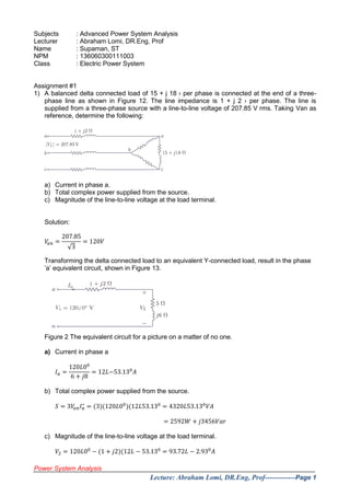
1. Power System Analysis
Lecture: Abraham Lomi, DR.Eng, Prof-------------Page 1
Subjects : Advanced Power System Analysis
Lecturer : Abraham Lomi, DR.Eng, Prof
Name : Supaman, ST
NPM : 136060300111003
Class : Electric Power System
Assignment #1
1) A balanced delta connected load of 15 + j 18 › per phase is connected at the end of a three- phase line as shown in Figure 12. The line impedance is 1 + j 2 › per phase. The line is supplied from a three-phase source with a line-to-line voltage of 207.85 V rms. Taking Van as reference, determine the following:
a) Current in phase a.
b) Total complex power supplied from the source.
c) Magnitude of the line-to-line voltage at the load terminal.
Solution:
푉푎푛= 207.85√3=120푉
Transforming the delta connected load to an equivalent Y-connected load, result in the phase ’a’ equivalent circuit, shown in Figure 13.
Figure 2 The equivalent circuit for a picture on a matter of no one.
a) Current in phase a
퐼푎= 120퐿006+푗8=12퐿−53.130퐴
b) Total complex power supplied from the source.
푆=3푉푎푛퐼푎∗ =(3)(120퐿00)(12퐿53.130=4320퐿53.130푉퐴
=2592푊+푗3456푉푎푟
c) Magnitude of the line-to-line voltage at the load terminal.
푉2=120퐿00−(1+푗2)(12퐿−53.130=93.72퐿−2.930퐴

2. Power System Analysis
Lecture: Abraham Lomi, DR.Eng, Prof-------------Page 2
Thus, the magnitude of the voltage line- to- line load terminals are :
푉퐿=√3(93.72)=162.3푉
Assignment #2
1) A 69-kV, three-phase short transmission line is 16 km long. The line has a per-phase series impedance of 0.125+j0.4375 Ω per km. Determine the sending end voltage, voltage regulation, the sending end power, and the transmission efficiency when the line delivers
a) 70 MVA, 0.8 lagging power factor at 64 kV
b) 120 MW, unity power factor at 64 kV
Solution:
The line impedance is
푍=(0,125+푗0,4375)푥(16)=2+푗7 Ω
The receiving end voltage per phase is
푉푅= 64퐿00√3=36,9504∟00퐾푣
a) The complex power at the receiving end is
푆푅(3∅)=70 ∠ 푐표푠−1푥 0,8=70 ∠36,870=56+푗42 푀푣푎
The current per phase is given by
퐼푅= 푆푅(3∅) ∗ 3푉푅 ∗= 70000∠−36,8703푥36,9504∠00=631,477∠−36,870퐴
The sending end voltage is
푉푆=푉푅+푍퐼푅
푉푆=푉푅+푍퐼푅=36,9504∠00+(2+푗7)푥(631,477∠−36,870)푥(10−3)
=40,708∠3,91370푘푉
The sending end line-to-line voltage magnitude is
|푉푆(퐿−퐿)|=√3|푉푆|
|푉푆(퐿−퐿)|=√3|40,708∟3,9137|=70,508 푘푉
The sending end power is
푆푆(3∅)=3푉푠퐼푆 ∗=3푥40,708∠3,91370푥 631,477∠−36,870푥10−3
=58,393 푀푊+푗50,374 푀푣푎푟
=77,1185 ∠ 40,7837 푀푉퐴

3. Power System Analysis
Lecture: Abraham Lomi, DR.Eng, Prof-------------Page 3
Voltage regulation is
Percent 푉푅= 70.508−6464 푥 100 %=10.169 %
Transmission line efciency is
ɳ= 푃푅(3∅) 푃푆(3∅) = 5658,393 푥100%=95,90%
b) The complex power at the receiving end is
푆푅(3∅)=120∟00=120+푗0 푀푉퐴
The current per phase is given by
퐼푅= 푆푅(3∅) ∗ 3푉푅 ∗= 12000∠003푥36,9504∠00=1082,53∠00퐴
The sending end voltage is
푉푠=푉푅+푍퐼푅=36,9504∠00+(2+푗7)푥 1082,53∠00푥(10)−3
=39,8427 ∠10,96390 푘푉
The sending end line-to-line voltage magnitude is
|푉푆(퐿−퐿)|=√3|푉푆|
|푉푆(퐿−퐿)|=√3|39,8427 ∠10,96390|=69,0096 푘푉
The sending end power is
푆푆(3∅)=3푉푆퐼푆 ∗=3푥39,8427 ∠10,96390푥1082,53∠00푥(10)−3
=127,031 푀푊+푗24,609 푀푣푎푟
=129,393 ∠ 10,96390 푀푉퐴
Voltage regulation is
푃푒푟푐푒푛푡 푉푅= 69,0096−6464 푥 100 %=7,8275 %
Transmission line efficiency is
ɳ= 푃푅(3∅) 푃푆(3∅) = 120127,031 푥100%=94,465%
Assignment #2 (cont’d)
2) A three-phase, 765-kV, 60-Hz transposed line is composed of four ACSR 1,431,000, 45/7 Bobolink conductors per phase with flat horizontal spacing of 14 m. The conductors have a diameter of 3.625 cm and a GMR of 1.439 cm. The bundle spacing is 45 cm. The line is 400 Km long, and for the purpose of this problem, a lossless line is assumed.

4. Power System Analysis
Lecture: Abraham Lomi, DR.Eng, Prof-------------Page 4
a) Determine the transmission line surge impedance Zc, phase constant β, wave length 휆, the surge impedance loading SIL, and the ABCD constant.
b) The line delivers 2000 MVA at 0.8 lagging power factor at 735 kV. Determine the sending end quantities and voltage regulation.
c) Determine the receiving end quantities when 1920 MW and 600 Mvar are being transmitted at 765 kV at the sending end.
d) The line is terminated in a purely resistive load. Determine the sending end quantities and voltage regulation when the receiving end load resistance is 264.5Ω at 735 kV.
Solution:
a) For hand calculation we have
퐺푀퐷=√(14)푥(14)푥(28)3=17,6389 푚
퐺푀푅퐿=1,09√(45)3푥(1,439)4=20.75 푐푚
퐺푀푅퐶=1,09√(45)3푥3,6252⁄4=21.98 푐푚
퐿=0,217,638920,75 푥 10−2=0,8885 푚퐻퐾푚⁄
퐶= 0,0556 푙푛 17,638921,98푥10−2=0,01268 휇퐹/퐾푚
The ABCD constants of the line are
퐴=cos훽ℓ=cos290=0,8746
퐵=푗푍푐sin훽ℓ=푗264,7sin290=푗128,33
퐶=푗 1 푍푐 sin훽ℓ=푗 1264,7sin290=푗0,0018315
퐷=퐴
b) The complex power at the receiving end is
푆푅(3∅)=2000 ∠36,870=1600 푀푊+푗1200 푀푣푎푟
푉푅= 735 ∠00√3=424,352 ∠ 00 푘푉
The current per phase is given by
퐼푅= 푆푅(3∅) ∗ 3푉푅 ∗= 2000000 ∠−36,8703푥424,352∠00=1571,02∠−36,870퐴

5. Power System Analysis
Lecture: Abraham Lomi, DR.Eng, Prof-------------Page 5
The sending end voltage is 푉푠=퐴푉푅+퐵퐼푅=0,8746 푥 424,352∠00+푗128,33 푥 1571,02 푥 10−3∠36,870
=517,86 ∠18,1470 푘푉
The sending end line-to-line voltage magnitude is |푉푆(퐿−퐿)|=√3|푉푆|
|푉푆(퐿−퐿)|=√3|517,86 ∠18,1470|=896,96 푘푉 훽=휔√퐿퐶
훽=2휋푥60√0,88853 푥 0,01268 푥 10−9 =0,001265 푅푎푑푖푎푛/퐾푚
훽ℓ=(0,001265 푥 400) 푥 (180휋⁄)=290
휆= 2휋 훽 = 2휋 0,001265=4967 퐾푚
푍퐶=√ 퐿 퐶 =√ 0,88853 푥 10−30,01268 푥 10−6=264,7 Ω
푆퐼퐿= (퐾푉퐿푅푎푡푒푑)2 푍퐶 = (765)2264,7=2210,89
The sending end current is
퐼푆=퐶푉푅+퐷퐼푅=푗0,0018315 푥 424352 ∠00+0,8746 푥 1571,02 ∠−36,870 =1100,23 ∠−2,460
The sending end power is
푆푆(3∅)=3푉푆퐼푆 ∗=3푥517,86 ∠18,1470푥1100,23∠2,460푥(10)−3
=1600 푀푊+푗601,59 푀푣푎푟
=1709,3 ∠ 20,60 푀푉퐴
Voltage regulation is
푃푒푟푐푒푛푡 푉푅= 896,960,8746−735735 푥 100 %=39,53 %
c) The complex power at the sending end is
푆푆(3∅)=1920 푀푊+푗600 푀푣푎푟=2011,566 ∠−17,3540 푀푉퐴
푉푆= 765 ∠00√3=441,673∠00

6. Power System Analysis
Lecture: Abraham Lomi, DR.Eng, Prof-------------Page 6
The sending end current per phase is given by
퐼푆= 푆푆(3∅) ∗ 3푉푆 ∗= 2011,566 ∠−17,35403푥441,673∠00=1518,14∠−17,3540퐴
The receiving end voltage is
푉푅=퐷푉푆−퐵퐼푆=0,8746 푥 441,673 ∠00−푗128,33 푥 1518,14 푥 10−3∠−17,3540=377,2 ∠−29,5370 푘푉
The receiving end line-to-line voltage magnitude is
|푉푅(퐿−퐿)|=√3|푉푆|
|푉푅(퐿−퐿)|=√3|377,2 ∠−29,5370|=653,33 푘푉
퐼푅=−퐶푉푆+퐴퐼푆=−푗0,0018315 푥 441673∠00+0,8746 푥 1518,14 ∠−17,3540=1748,73 ∠43,550 퐴
The receiving end power is
푆푅(3∅)=3푉푅퐼푅∗ =3푥377,2 ∠−29,5370 푥 1748,73 ∠43,55010−3 =1920 푀푊+푗479,2 푀푣푎푟 =1978,86 ∠ 14,0130 푀푉퐴
Voltage regulation is 푃푒푟푐푒푛푡 푉푅= 7650,8746−653,33653,33 푥 100 %=33,88 %
푉푅= 735∠00√3=424,352∠00 푘푉
The receiving end current per phase is given by 퐼푅= 푉푅 푍퐿 = 424352∠00264,5=1604,357∠00 퐴
The complex power at the receiving end is
푆푅(3∅)=3푉푅퐼푅∗ =3푥424,352 ∠00 푥 1604,357 ∠00 푥 10−3=2042,44 푀푊
The sending end voltage is 푉푆=퐴푉푅+퐵퐼푅=0,8746 푥 424,352 ∠00+푗128,33 푥 1604,357 푥 10−3∠00=424,42 ∠29,020 푘푉
The sending end line-to-line voltage magnitude is
|푉푆(퐿−퐿)|=√3|푉푆|

7. Power System Analysis
Lecture: Abraham Lomi, DR.Eng, Prof-------------Page 7
|푉푆(퐿−퐿)|=√3|424,42 ∠29,020|=735,12 푘푉
The sending end current is
퐼푆=퐶푉푅+퐷퐼푅=푗0,0018315 푥 424352∠00+0,8746 푥 1604,357 ∠00=1604,04 ∠28,980 퐴
푆푆(3∅)=3푉푆퐼푆 ∗=3푥424,42 ∠29,020 푥 1604,04 ∠−28,980 푥 10−3=2042,44 푀푊+푗1,4 푀푣푎푟 =2042,36 ∠0,040 푀푉퐴
Voltage regulation is
푃푒푟푐푒푛푡 푉푅= 735,120,8746−735735 푥 100 %=14,36 %
Assignment #3
3) A three-phase 420-kV, 60-Hz transmission line is 463 km long and may be assumed lossless. The line is energized with 420 kV at the sending end. When the load at the receiving end is removed, the voltage at the receiving end is 700 kV, and the per phase sending end current is 646.6∟90A.
a) Find the phase constant β in radians per km and the surge impedance Zc in Ω.
b) Ideal reactors are to be installed at the receiving end to keep |V| = |V| = 420 kV when load is removed. Determine the reactance per phase and the required three-phase Mvar.
Solution:
a) The sending end and receiving end voltages per phase are
푉푠= 420√3=242,487 푘푣 푉푅푛푙= 700√3=404,145 푘푣
With load removed 퐼푅=0,푓푟표푚 (5.71) we have 242,487=cos훽푙 푥 404,145 훽푙=53,130=0,927295 푅푎푑푖푎푛
And from (5.72), we have 푗646,6=푗 1 푍푐 =sin53,130푥 404,145 푥 103 푍푐=500 Ω
b) For 푉푠=푉푅 the required inductor reactance given by (5.100) is
푋푙푠ℎ= sin53,1301−cos53,130푥500=1000 Ω
The three-phase shunt reactor rating is 푄3휃=( 퐾푉퐿푅푎푡푒푑 푋퐿푠ℎ ) 2= 42021000=176,4 푀푣푎푟