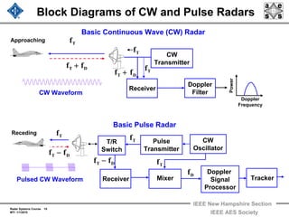
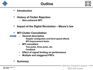
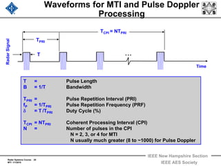
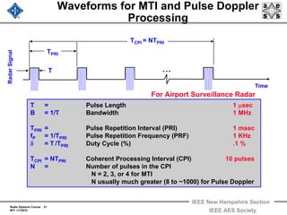
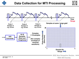
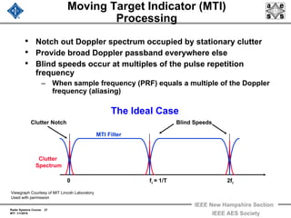
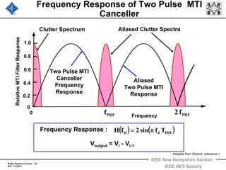
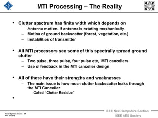
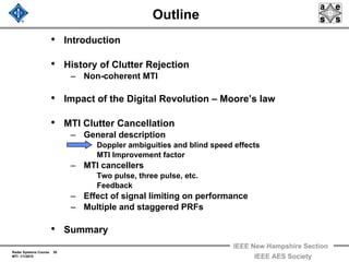
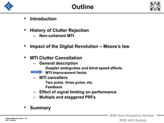
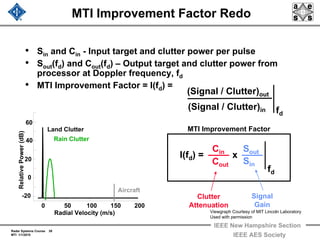
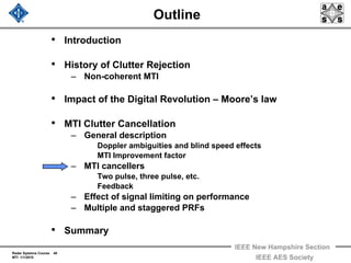
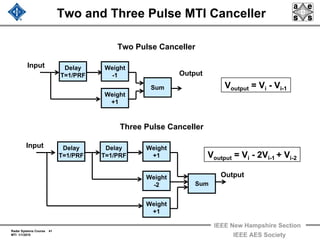
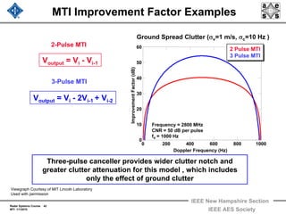
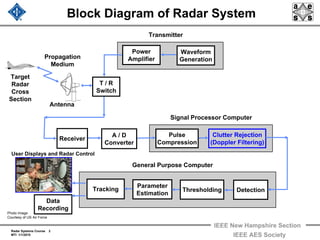
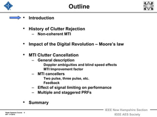
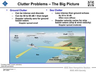
IEEE New Hampshire Section
Radar Systems Course 1
MTI 1/1/2010 IEEE AES Society
Radar Systems Engineering
Lecture 12
Clutter Rejection
Part 1 - Basics and Moving Target Indication
Dr. Robert M. O’Donnell
IEEE New Hampshire Section
Guest Lecturer
Radar Systems Course 2
MTI 1/1/2010
IEEE New Hampshire Section
IEEE AES Society
Pulse
Compression
Receiver
Clutter Rejection
(Doppler Filtering)
A / D
Converter
Block Diagram of Radar System
Antenna
Propagation
Medium
Target
Radar
Cross
Section
Transmitter
General Purpose Computer
Tracking
Data
Recording
Parameter
Estimation
Waveform
Generation
Detection
Power
Amplifier
T / R
Switch
Signal Processor Computer
Thresholding
User Displays and Radar Control
Photo Image
Courtesy of US Air Force
Radar Systems Course 3
MTI 1/1/2010
IEEE New Hampshire Section
IEEE AES Society
How to Handle Noise and Clutter
Viewgraph courtesy of MIT Lincoln Laboratory
Used with permission
Radar Systems Course 4
MTI 1/1/2010
IEEE New Hampshire Section
IEEE AES Society
How to Handle Noise and Clutter
If he doesn’t
take his arm off
my shoulder
I’m going to hide
his stash of
Hershey Bars !! Why does Steve
always talk me into doing
ridiculous
stunts like this ?
Viewgraph courtesy of MIT Lincoln Laboratory
Used with permission
Radar Systems Course 5
MTI 1/1/2010
IEEE New Hampshire Section
IEEE AES Society
Outline
• Introduction
• History of Clutter Rejection
– Non-coherent MTI
• Impact of the Digital Revolution – Moore’s law
• MTI Clutter Cancellation
– General description
Doppler ambiguities and blind speed effects
MTI Improvement factor
– MTI cancellers
Two pulse, three pulse, etc.
Feedback
– Effect of signal limiting on performance
– Multiple and staggered PRFs
• Summary
Radar Systems Course 6
MTI 1/1/2010
IEEE New Hampshire Section
IEEE AES Society
Clutter Problems – The Big Picture
• Ground Clutter
– Can be intense and discrete
– Can be 50 to 60 dB > than target
– Doppler velocity zero for ground
based radars
Doppler spread small
Bird
Flock Rain
Sea
Chaff
Ground
Urban Buildings
Targets
Ground
Hills
• Sea Clutter
– Less intense than ground echoes
By 20 to 30 dB
Often more diffuse
– Doppler velocity varies for ship
based radars (ship & wind velocity)
Doppler spread moderate
Courtesy of MIT Lincoln Laboratory
Used with permission
Radar Systems Course 7
MTI 1/1/2010
IEEE New Hampshire Section
IEEE AES Society
Clutter Problems – The Big Picture (cont.)
• Rain Clutter
– Diffuse and windblown
– Can be 30 dB > than target
Strength frequency dependant
– Mean Doppler varies relative to
wind direction & radar velocity
Doppler spread moderate
Bird
Flock Rain
Sea
Chaff
Ground
Urban Buildings
Targets
Ground
Hills
• Bird Clutter
– 100s to 10,000s of point targets
– Doppler velocity - 0 to 60 knots
Flocks of birds can fill 0 to 60 knots of
Doppler space
Big issue for very small targets
Courtesy of MIT Lincoln Laboratory
Used with permission
Radar Systems Course 8
MTI 1/1/2010
IEEE New Hampshire Section
IEEE AES Society
Example – Radar Display with Clutter
PPI Display of Heavy Rain
Courtesy of FAA
Radar Systems Course 9
MTI 1/1/2010
IEEE New Hampshire Section
IEEE AES Society
The Solution
Bird
Flock Rain
Sea
Chaff
Ground
Urban Buildings
Targets
Ground
Hills
• Moving Target Indicator (MTI) and Pulse-Doppler (PD)
processing use the Doppler shift of the different signals to
enhance detection of moving targets and reject clutter.
– The total solution is a sequential set of Doppler processing and
detection / thresholding techniques
• Smaller targets require more clutter suppression
Courtesy of MIT Lincoln Laboratory
Used with permission
Radar Systems Course 10
MTI 1/1/2010
IEEE New Hampshire Section
IEEE AES Society
The Doppler Effect
Transmitted Signal:
Received Signal:
( ) ( ) ( )tf2jexptAts 0T π=
( ) ( ) ( )[ ]tff2jexptAts D0R +πτ−α=
c
R2 0
=τ
λ
==
V2
c
fV2
f 0
D
Time Delay Doppler Frequency
( ) VtRtR 0 −=
Transmitted
Signal
Received
Signal Target
+ Approaching targets
- Receding targets
• The amplitude of the backscattered
signal is very weak
• The frequency of the received signal
is shifted by the Doppler Effect
• The delay of the received echo is
proportional to the distance to the target
Radar Systems Course 11
MTI 1/1/2010
IEEE New Hampshire Section
IEEE AES Society
Terminology & Basics
• Moving Target Indicator (MTI) Techniques
– Suppress clutter with a low pass Doppler filter
Reject slow moving clutter
Detect moving targets
– Small number of pulses typically used
Two to three pulses
– No estimate of target’s velocity
• Pulsed Doppler (PD) Techniques
– Suppress clutter with a set pass band Doppler filters
– Targets sorted into one or more Doppler filters
Targets radial velocity estimated
– A large number of pulses are coherently processed to generate
optimally shaped Doppler filters
From 10s to 1000s of pulses
• In this lecture Moving Target Indicator (MTI) techniques will
be studied
Radar Systems Course 12
MTI 1/1/2010
IEEE New Hampshire Section
IEEE AES Society
Outline
• Introduction
• History of Clutter Rejection
– Non-coherent MTI
• Impact of the Digital Revolution – Moore’s law
• MTI Clutter Cancellation
– General description
Doppler ambiguities and blind speed effects
MTI Improvement factor
– MTI cancellers
Two pulse, three pulse, etc.
Feedback
– Effect of signal limiting on performance
– Multiple and staggered PRFs
• Summary
Radar Systems Course 13
MTI 1/1/2010
IEEE New Hampshire Section
IEEE AES Society
Early Non Coherent MTI
• The earliest clutter (ground backscatter) rejection
technique consisted of storing an entire pulse of radar
echoes and subtracting it from the next pulse of echoes
– The storage devices were very crude by today’s standards
Plan Position Indicator (PPI) Display
Map-like Display
Radial distance to center Range
Angle of radius vector Azimuth
Threshold crossings Detections
Stationary Ground Echoes
Moving Aircraft Targets
PPI movie Courtesy of Flyingidiot
Courtesy of FAA
Radar Systems Course 14
MTI 1/1/2010
IEEE New Hampshire Section
IEEE AES Society
Block Diagrams of CW and Pulse Radars
Basic Continuous Wave (CW) Radar
Basic Pulse Radar
CW
Transmitter
T/R
Switch
Doppler
Filter
Doppler
Signal
Processor
Pulse
Transmitter
Power
Doppler
Frequency
Receiver
Tf
DT ff ±
Tf
DT ff ± Tf
Mixer
Tf CW
Oscillator
Receiver Tracker
DT ff ± Tf
Df
CW Waveform
Pulsed CW Waveform
Tf
DT ff ±
Radar Systems Course 15
MTI 1/1/2010
IEEE New Hampshire Section
IEEE AES Society
Block Diagrams of CW and Pulse Radars
Basic Continuous Wave (CW) Radar
Basic Pulse Radar
CW
Transmitter
T/R
Switch
Doppler
Filter
Doppler
Signal
Processor
Pulse
Transmitter
Power
Doppler
Frequency
Receiver
Tf
DT ff +
Tf
DT ff + Tf
Mixer
Tf CW
Oscillator
Receiver Tracker
DT ff − Tf
Df
CW Waveform
Pulsed CW Waveform
Tf
DT ff −
Approaching
Receding
Radar Systems Course 16
MTI 1/1/2010
IEEE New Hampshire Section
IEEE AES Society
Clutter Rejection History
• 1960s to mid 1970s
– Stability was a real problem
– Delay line cancellers
Several milliseconds delay
Quartz and mercury
Velocity of acoustic waves is 1/10,000 that of electromagnetic
waves
Disadvantages
Secondary waves
Large insertion waves
Dynamic range limitations of analog displays caused signals to
be limited
• Mid 1970s to present
– Revolution in digital technology
Memory capacity and processor speed continually increase, while
cost spirals downward
Affordable complex signal processing more and more easy and
less expensive to implement
Radar Systems Course 17
MTI 1/1/2010
IEEE New Hampshire Section
IEEE AES Society
Outline
• Introduction
• History of Clutter Rejection
– Non-coherent MTI
• Impact of the Digital Revolution – Moore’s law
• MTI Clutter Cancellation
– General description
Doppler ambiguities and blind speed effects
MTI Improvement factor
– MTI cancellers
Two pulse, three pulse, etc.
Feedback
– Effect of signal limiting on performance
– Multiple and staggered PRFs
• Summary
Radar Systems Course 18
MTI 1/1/2010
IEEE New Hampshire Section
IEEE AES Society
A Technology Perspective
• Three technologies have evolved and revolutionized radar
processing over the past 40 to 50 years
– Coherent transmitters
– A/D converter developments
High sample rate, linear, wide dynamic range
– The digital processing revolution - Moore’s law
- Low cost and compact digital memory and processors
– The development of the algorithmic formalism to practically
use this new digital hardware
“Digital Signal Processing”
• These developments have been the ‘technology enablers’
that have been key to the development the modern clutter
rejection techniques in today’s radar systems
Radar Systems Course 19
MTI 1/1/2010
IEEE New Hampshire Section
IEEE AES Society
Outline
• Introduction
• History of Clutter Rejection
– Non-coherent MTI
• Impact of the Digital Revolution – Moore’s law
• MTI Clutter Cancellation
– General description
Doppler ambiguities and blind speed effects
MTI Improvement factor
– MTI cancellers
Two pulse, three pulse, etc.
Feedback
– Effect of signal limiting on performance
– Multiple and staggered PRFs
• Summary
Radar Systems Course 20
MTI 1/1/2010
IEEE New Hampshire Section
IEEE AES Society
Waveforms for MTI and Pulse Doppler
Processing
T = Pulse Length
B = 1/T Bandwidth
TPRI = Pulse Repetition Interval (PRI)
fP = 1/TPRI Pulse Repetition Frequency (PRF)
δ = T /TPRI Duty Cycle (%)
TCPI = NTPRI Coherent Processing Interval (CPI)
N = Number of pulses in the CPI
N = 2, 3, or 4 for MTI
N usually much greater (8 to ~1000) for Pulse Doppler
TCPI = NTPRI
TPRI
T
Time
RadarSignal
• • •
Radar Systems Course 21
MTI 1/1/2010
IEEE New Hampshire Section
IEEE AES Society
Waveforms for MTI and Pulse Doppler
Processing
TCPI = NTPRI
TPRI
T
Time
RadarSignal
• • •
For Airport Surveillance Radar
T = Pulse Length 1 μsec
B = 1/T Bandwidth 1 MHz
TPRI = Pulse Repetition Interval (PRI) 1 msec
fP = 1/TPRI Pulse Repetition Frequency (PRF) 1 KHz
δ = T /TPRI Duty Cycle (%) .1 %
TCPI = NTPRI Coherent Processing Interval (CPI) 10 pulses
N = Number of pulses in the CPI
N = 2, 3, or 4 for MTI
N usually much greater (8 to ~1000) for Pulse Doppler
Radar Systems Course 22
MTI 1/1/2010
IEEE New Hampshire Section
IEEE AES Society
Data Collection for MTI Processing
Samples at same ‘range gate’
Sample No.
Range
PulseNumber
(Slowtime)
1
1 L
M
Time
Range
I & Q
Samples
(Real and
Imaginary)
Complex
I / Q samples
(the complex
envelope of
received
waveform)
Pulse 1
Sample 13
e.g. 4.6 km
Pulse 3
Sample 13
e.g. 4.6 km
Pulse 2
Sample 13
e.g. 4.6 km
A/D
Converter
Radar Systems Course 23
MTI 1/1/2010
IEEE New Hampshire Section
IEEE AES Society
Data Collection for MTI Processing
Samples at 13th ‘range gate’
Sample No.
Range
PulseNumber
(Slowtime)
1
1 L
M
Time
Range
I & Q
Samples
(Real and
Imaginary)
Complex
I / Q samples
(the complex
envelope of
received
waveform)
Pulse 1
Sample 13
e.g. 4.6 km
Pulse 3
Sample 13
e.g. 4.6 km
Pulse 2
Sample 13
e.g. 4.6 km
A/D
Converter
3
2
1
Radar Systems Course 24
MTI 1/1/2010
IEEE New Hampshire Section
IEEE AES Society
Range Ambiguities
Unambiguous Range
• Range ambiguous detections occur
when echoes from one pulse are not
all received before the next pulse
• Strong close targets (clutter) can
mask far weak targets
True
Range
Measured Radar
Range
Target 1
R1 R R Ru2 1
= +
Target 2
PRF
PRI
U
f2
c
2
Tc
R ==
Transmit
Pulse 1
Transmit
Pulse 2
Transmit
Pulse 3
Radar Systems Course 25
MTI 1/1/2010
IEEE New Hampshire Section
IEEE AES Society
Radar Range and Choice of PRF
Unambiguous Range vs.
Pulse Repetition Rate
UnambiguousRangeinnmi.
Pulse Repetition Rate (PRF) in KHz
.01 .02 .05 0.1 0.2 0.5 1.0 2.0 5.0 10.0
10
20
50
200
2,000
1,000
500
10,000
100
5,000
PRF
PRI
U
f2
c
2
Tc
R ==
• Unambiguous range is
inversely proportional
to the PRF.
• If the PRF is to high
“2nd time around”
clutter can be an issue
• ASR-9
– Range = 60 nmi
– PRF ≈ 1250 Hz
Radar Systems Course 26
MTI 1/1/2010
IEEE New Hampshire Section
IEEE AES Society
How MTI Works
Unprocessed
Radar Backscatter
Two Pulse MTI Canceller
Figure by MIT OCW.
Use low pass Doppler filter
to suppress clutter
backscatter
PPI Display
Input
Voutput = Vi - Vi-1
Delay
T=1/PRF
Sum
Output
Weight
+1
Weight
-1
Courtesy of FAA
Radar Systems Course 27
MTI 1/1/2010
IEEE New Hampshire Section
IEEE AES Society
Moving Target Indicator (MTI)
Processing
• Notch out Doppler spectrum occupied by stationary clutter
• Provide broad Doppler passband everywhere else
• Blind speeds occur at multiples of the pulse repetition
frequency
– When sample frequency (PRF) equals a multiple of the Doppler
frequency (aliasing)
0 fr = 1/T 2fr
Clutter Notch Blind Speeds
Clutter
Spectrum
MTI Filter
The Ideal Case
Viewgraph Courtesy of MIT Lincoln Laboratory
Used with permission
Radar Systems Course 28
MTI 1/1/2010
IEEE New Hampshire Section
IEEE AES Society
Frequency Response of Two Pulse MTI
Canceller
Frequency Response :
Aliased Clutter SpectraClutter Spectrum
Two Pulse MTI
Canceller
Frequency
Response
0
0
0.2
1.0
0.8
0.6
0.4
PRFf PRFf2Frequency
RelativeMTIFilterResponse
( ) ( )PRIdD Tfsin2fH π=
Adapted from Skolnik, reference 1
Voutput = Vi - Vi-1
Aliased
Two Pulse MTI
Response
Radar Systems Course 29
MTI 1/1/2010
IEEE New Hampshire Section
IEEE AES Society
MTI Processing – The Reality
• Clutter spectrum has finite width which depends on
– Antenna motion, if antenna is rotating mechanically
– Motion of ground backscatter (forest, vegetation, etc.)
– Instabilities of transmitter
• All MTI processors see some of this spectrally spread ground
clutter
– Two pulse, three pulse, four pulse etc, MTI cancellers
– Use of feedback in the MTI canceller design
• All of these have their strengths and weaknesses
– The main issue is how much clutter backscatter leaks through
the MTI Canceller
Called “Clutter Residue”
•
Radar Systems Course 30
MTI 1/1/2010
IEEE New Hampshire Section
IEEE AES Society
Outline
• Introduction
• History of Clutter Rejection
– Non-coherent MTI
• Impact of the Digital Revolution – Moore’s law
• MTI Clutter Cancellation
– General description
Doppler ambiguities and blind speed effects
MTI Improvement factor
– MTI cancellers
Two pulse, three pulse, etc.
Feedback
– Effect of signal limiting on performance
– Multiple and staggered PRFs
• Summary
Radar Systems Course 31
MTI 1/1/2010
IEEE New Hampshire Section
IEEE AES Society
Doppler Ambiguities
• Pulse Doppler waveform
samples target with sampling
rate = PRF
• Sampling causes aliasing at
multiples of PRF
• Two targets with Doppler
frequencies separated by an
integer multiple of the PRF
are indistinguishable
• Unambiguous velocity is
given by:
0
Sample Times
Moving V=Vu
Moving V=3Vu
Stationary V=0
2
f
V PRF
U
λ
=
PRFf PRFf2 PRFf3
PRFf
1
Viewgraph Courtesy of MIT Lincoln Laboratory
Used with permission
Radar Systems Course 32
MTI 1/1/2010
IEEE New Hampshire Section
IEEE AES Society
Blind Speed - Example
Doppler
Response
Radar Echo
Form target
Radar Echo
Form target
Radar Echo
Form target
• Blind Speeds, , result when the PRF ( ) is equal to
the target’s Doppler velocity (or a multiple of it)
• Doppler Velocity related to the Doppler Frequency by:
2
f
V D
D
λ
=
BV
egersintnVn
2
f
V B
PRF
U ±==
λ
=
PRFf
Radar Systems Course 33
MTI 1/1/2010
IEEE New Hampshire Section
IEEE AES Society
Unambiguous Doppler Velocity and Range
2
f
V PRF
B
λ
=
FirstBlindSpeed(knots)
10
30
100
1000
3000
300
Pulse Repetition Rate (KHz)
0.1 1 10 100
K a
Band
35
G
HzL
Band
1.3
G
Hz
U
HF
Band
435
G
Hz
VHF
Band
220
M
Hz
X
Band
9.4
G
Hz
S
Band
3.2
G
Hz
Radar Systems Course 34
MTI 1/1/2010
IEEE New Hampshire Section
IEEE AES Society
Unambiguous Doppler Velocity and Range
2
f
V PRF
B
λ
=
PRF
U
f2
c
R =
and
FirstBlindSpeed(knots)
10
30
100
1000
3000
300
Pulse Repetition Rate (KHz)
0.1 1 10 100
Unambiguous Range (nmi)
400 100 40 10 4 1
K a
Band
35
G
HzL
Band
1.3
G
Hz
U
HF
Band
435
G
Hz
X
Band
9.4
G
Hz
S
Band
3.2
G
HzVHF
Band
220
M
Hz
Radar Systems Course 35
MTI 1/1/2010
IEEE New Hampshire Section
IEEE AES Society
Unambiguous Doppler Velocity and Range
2
f
V PRF
B
λ
=
PRF
U
f2
c
R =
Combining
Yields
and
U
B
R4
c
V
λ
=
FirstBlindSpeed(knots)
10
30
100
1000
3000
300
Pulse Repetition Rate (KHz)
0.1 1 10 100
Unambiguous Range (nmi)
400 100 40 10 4 1
Example – ASR-9 knots120~VHz1250~fnmi60R BPRFU −−=
K a
Band
35
G
HzL
Band
1.3
G
Hz
U
HF
Band
435
G
Hz
X
Band
9.4
G
Hz
S
Band
3.2
G
HzVHF
Band
220
M
Hz
Radar Systems Course 36
MTI 1/1/2010
IEEE New Hampshire Section
IEEE AES Society
MTI Blind Phase Loss – Example 1
• In this case, after processing through a two pulse MTI, half
of the signal energy is lost if only the I channel is used
• Use of both I and Q channels will solve this problem
I Channel
Q Channel
1a 2a
3a 4a
5a 6a
0aa
0aa
0aa
0aa
54
43
32
21
≠−
=−
≠−
=−
1b
2b 3b
4b 5b
6b
0bb
0bb
0bb
0bb
54
43
32
21
=−
≠−
=−
≠−
Radar Systems Course 37
MTI 1/1/2010
IEEE New Hampshire Section
IEEE AES Society
• The PRF is twice the Doppler frequency of the target signal.
• The phase of the PRF is such that, for the I channel, sampling occurs at
zero crossings
• However, in the Q channel sampling, the signal is completely recovered,
again showing the need for implementation of both the I and Q channels
I Channel
Q Channel
MTI Blind Phase Loss – Example 2
2a 4a
3a1a 0aa
0aa
0aa
43
32
21
=−
=−
=−
Because all samples =0
1b
2b 4b
3b
0bb
0bb
0bb
43
32
21
≠−
≠−
≠−
Radar Systems Course 38
MTI 1/1/2010
IEEE New Hampshire Section
IEEE AES Society
Outline
• Introduction
• History of Clutter Rejection
– Non-coherent MTI
• Impact of the Digital Revolution – Moore’s law
• MTI Clutter Cancellation
– General description
Doppler ambiguities and blind speed effects
MTI Improvement factor
– MTI cancellers
Two pulse, three pulse, etc.
Feedback
– Effect of signal limiting on performance
– Multiple and staggered PRFs
• Summary
Radar Systems Course 39
MTI 1/1/2010
IEEE New Hampshire Section
IEEE AES Society
MTI Improvement Factor Redo
• Sin and Cin - Input target and clutter power per pulse
• Sout(fd) and Cout(fd) – Output target and clutter power from
processor at Doppler frequency, fd
• MTI Improvement Factor = I(fd) =
0 50 100 150 200
-20
0
20
40
60
Radial Velocity (m/s)
RelativePower(dB)
Land Clutter
Rain Clutter
Aircraft
(Signal / Clutter)out
(Signal / Clutter)in fd
I(fd) = x
fd
Cin
Cout Sin
Sout
Clutter
Attenuation
Signal
Gain
MTI Improvement Factor
Viewgraph Courtesy of MIT Lincoln Laboratory
Used with permission
Radar Systems Course 40
MTI 1/1/2010
IEEE New Hampshire Section
IEEE AES Society
Outline
• Introduction
• History of Clutter Rejection
– Non-coherent MTI
• Impact of the Digital Revolution – Moore’s law
• MTI Clutter Cancellation
– General description
Doppler ambiguities and blind speed effects
MTI Improvement factor
– MTI cancellers
Two pulse, three pulse, etc.
Feedback
– Effect of signal limiting on performance
– Multiple and staggered PRFs
• Summary
Radar Systems Course 41
MTI 1/1/2010
IEEE New Hampshire Section
IEEE AES Society
Two and Three Pulse MTI Canceller
Two Pulse Canceller
Delay
T=1/PRF
Sum
Input
Output
Voutput = Vi - Vi-1
Weight
+1
Weight
-1
Delay
T=1/PRF
Delay
T=1/PRF
Input
Weight
+1
Weight
-2
Weight
+1
Sum
Output
Voutput = Vi - 2Vi-1 + Vi-2
Three Pulse Canceller
Radar Systems Course 42
MTI 1/1/2010
IEEE New Hampshire Section
IEEE AES Society
MTI Improvement Factor Examples
Ground Spread Clutter (σv=1 m/s, σc=10 Hz )
0 200 400 600 800 1000
0
10
20
30
40
50
60
Doppler Frequency (Hz)
ImprovementFactor(dB)
2 Pulse MTI
3 Pulse MTI
2 Pulse MTI
3 Pulse MTI
Voutput = Vi - Vi-1
Voutput = Vi - 2Vi-1 + Vi-2
3-Pulse MTI
2-Pulse MTI
Frequency = 2800 MHz
CNR = 50 dB per pulse
fd = 1000 Hz
Three-pulse canceller provides wider clutter notch and
greater clutter attenuation for this model , which includes
only the effect of ground clutter
Viewgraph Courtesy of MIT Lincoln Laboratory
Used with permission
Radar Systems Course 43
MTI 1/1/2010
IEEE New Hampshire Section
IEEE AES Society
MTI Cancellers Employing Feedback
• With few pulses it is very difficult to develop a filter, which
has a rectangular shape without employing feedback in the
MTI canceller
τ
τ τ
∑ ∑∑∑∑
-1
-1
0.61
+1 +1
0.27
+1+1
0.04
INV
OUTV
-1
+1
Recursive MTI Filter Based on a Three Pole Chebyshev Design
0.0 0.5 PRF PRF 1.5 PRF
Filter Response
0.0
0.5
1.0
0.5 dB ripple
in passband
Radar Systems Course 44
MTI 1/1/2010
IEEE New Hampshire Section
IEEE AES Society
Recursive Techniques For MTI Cancellation
• Advantages
– Good rectangular response across Doppler spectrum
– Well suited for weather sensing radars, which want to reject
ground clutter and detect moving precipitation
NEXRAD (WSR-88)
Terminal Doppler Weather radar (TDWR)
• Disadvantages
– Poor rejection of moving clutter, such as rain or chaff
– Large discrete clutter echoes and interference from other
nearby radars can produce transient ringing in these
recursive filters
Avoided in military radars
Radar Systems Course 45
MTI 1/1/2010
IEEE New Hampshire Section
IEEE AES Society
Outline
• Introduction
• History of Clutter Rejection
– Non-coherent MTI
• Impact of the Digital Revolution – Moore’s law
• MTI Clutter Cancellation
– General description
Doppler ambiguities and blind speed effects
MTI Improvement factor
– MTI cancellers
Two pulse, three pulse, etc.
Feedback
– Effect of signal limiting on performance
– Multiple and staggered PRFs
• Summary
Radar Systems Course 46
MTI 1/1/2010
IEEE New Hampshire Section
IEEE AES Society
Use of Limiters in MTI Radars
• Before the days of modern A/D converters, with wide
dynamic range and high sample rate, radars needed to
apply a limiter to the radar signal in the receiver of
saturation would occur.
– Analog displays would “bloom” because they had only 20 db
or so dynamic range.
– Limiting of the amplitude of large clutter discrete echoes,
causes significant spread of their spectra
• Its has been shown that use of limiters with MTI cancellers
significantly reduces their performance
– MTI Improvement factor of a 3 pulse canceller is reduced from
42 db (without limiting) to 29 dB (with limiting)
• The modern and simple solution is to use A/D converters,
with enough bits, so that they can adequately
accommodate all of the expected signal and clutter echoes
within their dynamic range
Radar Systems Course 47
MTI 1/1/2010
IEEE New Hampshire Section
IEEE AES Society
Outline
• Introduction
• History of Clutter Rejection
– Non-coherent MTI
• Impact of the Digital Revolution – Moore’s law
• MTI Clutter Cancellation
– General description
Range and Doppler ambiguities; blind speed effects
MTI Improvement factor
– MTI cancellers
Two pulse, three pulse, etc.
Feedback
– Effect of signal limiting on performance
– Multiple and staggered PRFs
• Summary
Radar Systems Course 48
MTI 1/1/2010
IEEE New Hampshire Section
IEEE AES Society
Use of Multiple PRFs to Mitigate
Blind Speed Issues
• Using multiple PRFs allows targets, whose radial velocity corresponds
to the blind speed at 1 PRF, to be detected at another PRF.
• PRFs may be changed from scan to scan, dwell to dwell, or from pulse
to pulse (Staggered PRFs)
MTIResponse
0.0
1.0
MTIResponse
0.0
1.0
MTIResponse
0.0
1.0
Doppler Frequency
Doppler Frequency
Doppler Frequency
PRF1 3 PRF12 PRF1 4 PRF1
PRF2
MTI response
for PRF1
4 PRF23 PRF22 PRF2
5 PRF2
MTI response
for PRF1
Combined
MTI response
using both PRFs
PRF1 2 PRF2
3 PRF1
Note: 4 PRF1 = 5 PRF2
3 PRF2
Radar Systems Course 49
MTI 1/1/2010
IEEE New Hampshire Section
IEEE AES Society
Staggered PRFs to Increase Blind Speed
• Staggering or changing the time between pulses (Pulse
Repetition Rate - PRF) will raise the blind speed
• Although the staggered PRFs remove the blind speeds that
would have been obtained with a constant PRF, there will
eventually be a new blind speed
• This occurs when the PRFs have the following relationship:
• Where are relatively prime integers
• The ratio of the first blind speed, , with the staggered PRF
waveform to the first blind speed, , of a waveform with a
constant PRF is:
n
nn332211 ffff η=⋅⋅⋅=η=η=η
n,3,2,1 η⋅⋅⋅ηηη
( )
nv
v n321
B
1 η+⋅⋅⋅+η+η+η
=
1v
Bv
Radar Systems Course 50
MTI 1/1/2010
IEEE New Hampshire Section
IEEE AES Society
Staggered PRFs to Increase Blind Speed
0 100 200 300 400 500 600 700 800
-20
-10
0
Radial Velocity (m/s)
SNRRelativetoSinglePulse(dB)
0 100 200 300 400 500 600 700 800
-20
-10
0
Radial Velocity (m/s)
Fixed 2 kHz PRI at S-Band
Staggered 2 kHz, 1.754 kHz PRI
• Staggering or changing the
time between pulses will
raise the blind speed
• Although the staggered
PRF’s remove the blind
speeds that would have been
obtained with a constant
PRF, there will be a new
much higher blind speed
• Use of staggered PRFs does
not allow he MTI cancellation
of “2nd time around clutter”
MTI Frequency Response
Viewgraph Courtesy of MIT Lincoln Laboratory
Used with permission
Radar Systems Course 51
MTI 1/1/2010
IEEE New Hampshire Section
IEEE AES Society
Summary
• Moving Target Indicator (MTI) techniques are Doppler filtering
techniques that reject stationary clutter
– Radial velocity is not measured
• Blind speeds are regions of Doppler space where targets with
those Doppler velocities cannot be detected
• Two and three pulse MTI cancellers are examples of MTI filters
• Methods of increasing the blind speed
– Changing the time between groups of pulses (multiple PRFs)
– Changing the time between individual pulses (staggered PRFs)
– There are pros and cons to each of these techniques
• There is significant difficulty suppressing moving clutter (rain)
with MTI techniques
Radar Systems Course 52
MTI 1/1/2010
IEEE New Hampshire Section
IEEE AES Society
Homework Problems
• From Skolnik (Reference 1)
– Problems 3-1, 3-2, 3-3, 3-4, 3-5, 3-6 and 3-8
Radar Systems Course 53
MTI 1/1/2010
IEEE New Hampshire Section
IEEE AES Society
References
1. Skolnik, M., Introduction to Radar Systems, McGraw-Hill, New York,
3rd Ed., 2001
2. Barton, D. K., Modern Radar System Analysis, Norwood, Mass.,
Artech House, 1988
3. Skolnik, M., Editor in Chief, Radar Handbook, New York, McGraw-
Hill, 3rd Ed., 2008
4. Skolnik, M., Editor in Chief, Radar Handbook, New York, McGraw-
Hill, 2nd Ed., 1990
5. Nathanson, F. E., Radar Design Principles, New York, McGraw-Hill,
1st Ed., 1969
6. Richards, M., Fundamentals of Radar Signal Processing, McGraw-
Hill, New York, 2005
7. Schleher, D. C., MTI and Pulsed Doppler Radar, Artech, Boston,
1991
8. Bassford, R. et al, Test and Evaluation of the Moving Target
Detector (MTD) Radar, FAA Report, FAA-RD-77-118, 1977
Radar Systems Course 54
MTI 1/1/2010
IEEE New Hampshire Section
IEEE AES Society
Acknowledgements
• Mr. C. E. Muehe
• Dr. James Ward

Radar 2009 a 12 clutter rejection basics and mti

  • 1.
    IEEE New HampshireSection Radar Systems Course 1 MTI 1/1/2010 IEEE AES Society Radar Systems Engineering Lecture 12 Clutter Rejection Part 1 - Basics and Moving Target Indication Dr. Robert M. O’Donnell IEEE New Hampshire Section Guest Lecturer
  • 2.
    Radar Systems Course2 MTI 1/1/2010 IEEE New Hampshire Section IEEE AES Society Pulse Compression Receiver Clutter Rejection (Doppler Filtering) A / D Converter Block Diagram of Radar System Antenna Propagation Medium Target Radar Cross Section Transmitter General Purpose Computer Tracking Data Recording Parameter Estimation Waveform Generation Detection Power Amplifier T / R Switch Signal Processor Computer Thresholding User Displays and Radar Control Photo Image Courtesy of US Air Force
  • 3.
    Radar Systems Course3 MTI 1/1/2010 IEEE New Hampshire Section IEEE AES Society How to Handle Noise and Clutter Viewgraph courtesy of MIT Lincoln Laboratory Used with permission
  • 4.
    Radar Systems Course4 MTI 1/1/2010 IEEE New Hampshire Section IEEE AES Society How to Handle Noise and Clutter If he doesn’t take his arm off my shoulder I’m going to hide his stash of Hershey Bars !! Why does Steve always talk me into doing ridiculous stunts like this ? Viewgraph courtesy of MIT Lincoln Laboratory Used with permission
  • 5.
    Radar Systems Course5 MTI 1/1/2010 IEEE New Hampshire Section IEEE AES Society Outline • Introduction • History of Clutter Rejection – Non-coherent MTI • Impact of the Digital Revolution – Moore’s law • MTI Clutter Cancellation – General description Doppler ambiguities and blind speed effects MTI Improvement factor – MTI cancellers Two pulse, three pulse, etc. Feedback – Effect of signal limiting on performance – Multiple and staggered PRFs • Summary
  • 6.
    Radar Systems Course6 MTI 1/1/2010 IEEE New Hampshire Section IEEE AES Society Clutter Problems – The Big Picture • Ground Clutter – Can be intense and discrete – Can be 50 to 60 dB > than target – Doppler velocity zero for ground based radars Doppler spread small Bird Flock Rain Sea Chaff Ground Urban Buildings Targets Ground Hills • Sea Clutter – Less intense than ground echoes By 20 to 30 dB Often more diffuse – Doppler velocity varies for ship based radars (ship & wind velocity) Doppler spread moderate Courtesy of MIT Lincoln Laboratory Used with permission
  • 7.
    Radar Systems Course7 MTI 1/1/2010 IEEE New Hampshire Section IEEE AES Society Clutter Problems – The Big Picture (cont.) • Rain Clutter – Diffuse and windblown – Can be 30 dB > than target Strength frequency dependant – Mean Doppler varies relative to wind direction & radar velocity Doppler spread moderate Bird Flock Rain Sea Chaff Ground Urban Buildings Targets Ground Hills • Bird Clutter – 100s to 10,000s of point targets – Doppler velocity - 0 to 60 knots Flocks of birds can fill 0 to 60 knots of Doppler space Big issue for very small targets Courtesy of MIT Lincoln Laboratory Used with permission
  • 8.
    Radar Systems Course8 MTI 1/1/2010 IEEE New Hampshire Section IEEE AES Society Example – Radar Display with Clutter PPI Display of Heavy Rain Courtesy of FAA
  • 9.
    Radar Systems Course9 MTI 1/1/2010 IEEE New Hampshire Section IEEE AES Society The Solution Bird Flock Rain Sea Chaff Ground Urban Buildings Targets Ground Hills • Moving Target Indicator (MTI) and Pulse-Doppler (PD) processing use the Doppler shift of the different signals to enhance detection of moving targets and reject clutter. – The total solution is a sequential set of Doppler processing and detection / thresholding techniques • Smaller targets require more clutter suppression Courtesy of MIT Lincoln Laboratory Used with permission
  • 10.
    Radar Systems Course10 MTI 1/1/2010 IEEE New Hampshire Section IEEE AES Society The Doppler Effect Transmitted Signal: Received Signal: ( ) ( ) ( )tf2jexptAts 0T π= ( ) ( ) ( )[ ]tff2jexptAts D0R +πτ−α= c R2 0 =τ λ == V2 c fV2 f 0 D Time Delay Doppler Frequency ( ) VtRtR 0 −= Transmitted Signal Received Signal Target + Approaching targets - Receding targets • The amplitude of the backscattered signal is very weak • The frequency of the received signal is shifted by the Doppler Effect • The delay of the received echo is proportional to the distance to the target
  • 11.
    Radar Systems Course11 MTI 1/1/2010 IEEE New Hampshire Section IEEE AES Society Terminology & Basics • Moving Target Indicator (MTI) Techniques – Suppress clutter with a low pass Doppler filter Reject slow moving clutter Detect moving targets – Small number of pulses typically used Two to three pulses – No estimate of target’s velocity • Pulsed Doppler (PD) Techniques – Suppress clutter with a set pass band Doppler filters – Targets sorted into one or more Doppler filters Targets radial velocity estimated – A large number of pulses are coherently processed to generate optimally shaped Doppler filters From 10s to 1000s of pulses • In this lecture Moving Target Indicator (MTI) techniques will be studied
  • 12.
    Radar Systems Course12 MTI 1/1/2010 IEEE New Hampshire Section IEEE AES Society Outline • Introduction • History of Clutter Rejection – Non-coherent MTI • Impact of the Digital Revolution – Moore’s law • MTI Clutter Cancellation – General description Doppler ambiguities and blind speed effects MTI Improvement factor – MTI cancellers Two pulse, three pulse, etc. Feedback – Effect of signal limiting on performance – Multiple and staggered PRFs • Summary
  • 13.
    Radar Systems Course13 MTI 1/1/2010 IEEE New Hampshire Section IEEE AES Society Early Non Coherent MTI • The earliest clutter (ground backscatter) rejection technique consisted of storing an entire pulse of radar echoes and subtracting it from the next pulse of echoes – The storage devices were very crude by today’s standards Plan Position Indicator (PPI) Display Map-like Display Radial distance to center Range Angle of radius vector Azimuth Threshold crossings Detections Stationary Ground Echoes Moving Aircraft Targets PPI movie Courtesy of Flyingidiot Courtesy of FAA
  • 14.
    Radar Systems Course14 MTI 1/1/2010 IEEE New Hampshire Section IEEE AES Society Block Diagrams of CW and Pulse Radars Basic Continuous Wave (CW) Radar Basic Pulse Radar CW Transmitter T/R Switch Doppler Filter Doppler Signal Processor Pulse Transmitter Power Doppler Frequency Receiver Tf DT ff ± Tf DT ff ± Tf Mixer Tf CW Oscillator Receiver Tracker DT ff ± Tf Df CW Waveform Pulsed CW Waveform Tf DT ff ±
  • 15.
    Radar Systems Course15 MTI 1/1/2010 IEEE New Hampshire Section IEEE AES Society Block Diagrams of CW and Pulse Radars Basic Continuous Wave (CW) Radar Basic Pulse Radar CW Transmitter T/R Switch Doppler Filter Doppler Signal Processor Pulse Transmitter Power Doppler Frequency Receiver Tf DT ff + Tf DT ff + Tf Mixer Tf CW Oscillator Receiver Tracker DT ff − Tf Df CW Waveform Pulsed CW Waveform Tf DT ff − Approaching Receding
  • 16.
    Radar Systems Course16 MTI 1/1/2010 IEEE New Hampshire Section IEEE AES Society Clutter Rejection History • 1960s to mid 1970s – Stability was a real problem – Delay line cancellers Several milliseconds delay Quartz and mercury Velocity of acoustic waves is 1/10,000 that of electromagnetic waves Disadvantages Secondary waves Large insertion waves Dynamic range limitations of analog displays caused signals to be limited • Mid 1970s to present – Revolution in digital technology Memory capacity and processor speed continually increase, while cost spirals downward Affordable complex signal processing more and more easy and less expensive to implement
  • 17.
    Radar Systems Course17 MTI 1/1/2010 IEEE New Hampshire Section IEEE AES Society Outline • Introduction • History of Clutter Rejection – Non-coherent MTI • Impact of the Digital Revolution – Moore’s law • MTI Clutter Cancellation – General description Doppler ambiguities and blind speed effects MTI Improvement factor – MTI cancellers Two pulse, three pulse, etc. Feedback – Effect of signal limiting on performance – Multiple and staggered PRFs • Summary
  • 18.
    Radar Systems Course18 MTI 1/1/2010 IEEE New Hampshire Section IEEE AES Society A Technology Perspective • Three technologies have evolved and revolutionized radar processing over the past 40 to 50 years – Coherent transmitters – A/D converter developments High sample rate, linear, wide dynamic range – The digital processing revolution - Moore’s law - Low cost and compact digital memory and processors – The development of the algorithmic formalism to practically use this new digital hardware “Digital Signal Processing” • These developments have been the ‘technology enablers’ that have been key to the development the modern clutter rejection techniques in today’s radar systems
  • 19.
    Radar Systems Course19 MTI 1/1/2010 IEEE New Hampshire Section IEEE AES Society Outline • Introduction • History of Clutter Rejection – Non-coherent MTI • Impact of the Digital Revolution – Moore’s law • MTI Clutter Cancellation – General description Doppler ambiguities and blind speed effects MTI Improvement factor – MTI cancellers Two pulse, three pulse, etc. Feedback – Effect of signal limiting on performance – Multiple and staggered PRFs • Summary
  • 20.
    Radar Systems Course20 MTI 1/1/2010 IEEE New Hampshire Section IEEE AES Society Waveforms for MTI and Pulse Doppler Processing T = Pulse Length B = 1/T Bandwidth TPRI = Pulse Repetition Interval (PRI) fP = 1/TPRI Pulse Repetition Frequency (PRF) δ = T /TPRI Duty Cycle (%) TCPI = NTPRI Coherent Processing Interval (CPI) N = Number of pulses in the CPI N = 2, 3, or 4 for MTI N usually much greater (8 to ~1000) for Pulse Doppler TCPI = NTPRI TPRI T Time RadarSignal • • •
  • 21.
    Radar Systems Course21 MTI 1/1/2010 IEEE New Hampshire Section IEEE AES Society Waveforms for MTI and Pulse Doppler Processing TCPI = NTPRI TPRI T Time RadarSignal • • • For Airport Surveillance Radar T = Pulse Length 1 μsec B = 1/T Bandwidth 1 MHz TPRI = Pulse Repetition Interval (PRI) 1 msec fP = 1/TPRI Pulse Repetition Frequency (PRF) 1 KHz δ = T /TPRI Duty Cycle (%) .1 % TCPI = NTPRI Coherent Processing Interval (CPI) 10 pulses N = Number of pulses in the CPI N = 2, 3, or 4 for MTI N usually much greater (8 to ~1000) for Pulse Doppler
  • 22.
    Radar Systems Course22 MTI 1/1/2010 IEEE New Hampshire Section IEEE AES Society Data Collection for MTI Processing Samples at same ‘range gate’ Sample No. Range PulseNumber (Slowtime) 1 1 L M Time Range I & Q Samples (Real and Imaginary) Complex I / Q samples (the complex envelope of received waveform) Pulse 1 Sample 13 e.g. 4.6 km Pulse 3 Sample 13 e.g. 4.6 km Pulse 2 Sample 13 e.g. 4.6 km A/D Converter
  • 23.
    Radar Systems Course23 MTI 1/1/2010 IEEE New Hampshire Section IEEE AES Society Data Collection for MTI Processing Samples at 13th ‘range gate’ Sample No. Range PulseNumber (Slowtime) 1 1 L M Time Range I & Q Samples (Real and Imaginary) Complex I / Q samples (the complex envelope of received waveform) Pulse 1 Sample 13 e.g. 4.6 km Pulse 3 Sample 13 e.g. 4.6 km Pulse 2 Sample 13 e.g. 4.6 km A/D Converter 3 2 1
  • 24.
    Radar Systems Course24 MTI 1/1/2010 IEEE New Hampshire Section IEEE AES Society Range Ambiguities Unambiguous Range • Range ambiguous detections occur when echoes from one pulse are not all received before the next pulse • Strong close targets (clutter) can mask far weak targets True Range Measured Radar Range Target 1 R1 R R Ru2 1 = + Target 2 PRF PRI U f2 c 2 Tc R == Transmit Pulse 1 Transmit Pulse 2 Transmit Pulse 3
  • 25.
    Radar Systems Course25 MTI 1/1/2010 IEEE New Hampshire Section IEEE AES Society Radar Range and Choice of PRF Unambiguous Range vs. Pulse Repetition Rate UnambiguousRangeinnmi. Pulse Repetition Rate (PRF) in KHz .01 .02 .05 0.1 0.2 0.5 1.0 2.0 5.0 10.0 10 20 50 200 2,000 1,000 500 10,000 100 5,000 PRF PRI U f2 c 2 Tc R == • Unambiguous range is inversely proportional to the PRF. • If the PRF is to high “2nd time around” clutter can be an issue • ASR-9 – Range = 60 nmi – PRF ≈ 1250 Hz
  • 26.
    Radar Systems Course26 MTI 1/1/2010 IEEE New Hampshire Section IEEE AES Society How MTI Works Unprocessed Radar Backscatter Two Pulse MTI Canceller Figure by MIT OCW. Use low pass Doppler filter to suppress clutter backscatter PPI Display Input Voutput = Vi - Vi-1 Delay T=1/PRF Sum Output Weight +1 Weight -1 Courtesy of FAA
  • 27.
    Radar Systems Course27 MTI 1/1/2010 IEEE New Hampshire Section IEEE AES Society Moving Target Indicator (MTI) Processing • Notch out Doppler spectrum occupied by stationary clutter • Provide broad Doppler passband everywhere else • Blind speeds occur at multiples of the pulse repetition frequency – When sample frequency (PRF) equals a multiple of the Doppler frequency (aliasing) 0 fr = 1/T 2fr Clutter Notch Blind Speeds Clutter Spectrum MTI Filter The Ideal Case Viewgraph Courtesy of MIT Lincoln Laboratory Used with permission
  • 28.
    Radar Systems Course28 MTI 1/1/2010 IEEE New Hampshire Section IEEE AES Society Frequency Response of Two Pulse MTI Canceller Frequency Response : Aliased Clutter SpectraClutter Spectrum Two Pulse MTI Canceller Frequency Response 0 0 0.2 1.0 0.8 0.6 0.4 PRFf PRFf2Frequency RelativeMTIFilterResponse ( ) ( )PRIdD Tfsin2fH π= Adapted from Skolnik, reference 1 Voutput = Vi - Vi-1 Aliased Two Pulse MTI Response
  • 29.
    Radar Systems Course29 MTI 1/1/2010 IEEE New Hampshire Section IEEE AES Society MTI Processing – The Reality • Clutter spectrum has finite width which depends on – Antenna motion, if antenna is rotating mechanically – Motion of ground backscatter (forest, vegetation, etc.) – Instabilities of transmitter • All MTI processors see some of this spectrally spread ground clutter – Two pulse, three pulse, four pulse etc, MTI cancellers – Use of feedback in the MTI canceller design • All of these have their strengths and weaknesses – The main issue is how much clutter backscatter leaks through the MTI Canceller Called “Clutter Residue” •
  • 30.
    Radar Systems Course30 MTI 1/1/2010 IEEE New Hampshire Section IEEE AES Society Outline • Introduction • History of Clutter Rejection – Non-coherent MTI • Impact of the Digital Revolution – Moore’s law • MTI Clutter Cancellation – General description Doppler ambiguities and blind speed effects MTI Improvement factor – MTI cancellers Two pulse, three pulse, etc. Feedback – Effect of signal limiting on performance – Multiple and staggered PRFs • Summary
  • 31.
    Radar Systems Course31 MTI 1/1/2010 IEEE New Hampshire Section IEEE AES Society Doppler Ambiguities • Pulse Doppler waveform samples target with sampling rate = PRF • Sampling causes aliasing at multiples of PRF • Two targets with Doppler frequencies separated by an integer multiple of the PRF are indistinguishable • Unambiguous velocity is given by: 0 Sample Times Moving V=Vu Moving V=3Vu Stationary V=0 2 f V PRF U λ = PRFf PRFf2 PRFf3 PRFf 1 Viewgraph Courtesy of MIT Lincoln Laboratory Used with permission
  • 32.
    Radar Systems Course32 MTI 1/1/2010 IEEE New Hampshire Section IEEE AES Society Blind Speed - Example Doppler Response Radar Echo Form target Radar Echo Form target Radar Echo Form target • Blind Speeds, , result when the PRF ( ) is equal to the target’s Doppler velocity (or a multiple of it) • Doppler Velocity related to the Doppler Frequency by: 2 f V D D λ = BV egersintnVn 2 f V B PRF U ±== λ = PRFf
  • 33.
    Radar Systems Course33 MTI 1/1/2010 IEEE New Hampshire Section IEEE AES Society Unambiguous Doppler Velocity and Range 2 f V PRF B λ = FirstBlindSpeed(knots) 10 30 100 1000 3000 300 Pulse Repetition Rate (KHz) 0.1 1 10 100 K a Band 35 G HzL Band 1.3 G Hz U HF Band 435 G Hz VHF Band 220 M Hz X Band 9.4 G Hz S Band 3.2 G Hz
  • 34.
    Radar Systems Course34 MTI 1/1/2010 IEEE New Hampshire Section IEEE AES Society Unambiguous Doppler Velocity and Range 2 f V PRF B λ = PRF U f2 c R = and FirstBlindSpeed(knots) 10 30 100 1000 3000 300 Pulse Repetition Rate (KHz) 0.1 1 10 100 Unambiguous Range (nmi) 400 100 40 10 4 1 K a Band 35 G HzL Band 1.3 G Hz U HF Band 435 G Hz X Band 9.4 G Hz S Band 3.2 G HzVHF Band 220 M Hz
  • 35.
    Radar Systems Course35 MTI 1/1/2010 IEEE New Hampshire Section IEEE AES Society Unambiguous Doppler Velocity and Range 2 f V PRF B λ = PRF U f2 c R = Combining Yields and U B R4 c V λ = FirstBlindSpeed(knots) 10 30 100 1000 3000 300 Pulse Repetition Rate (KHz) 0.1 1 10 100 Unambiguous Range (nmi) 400 100 40 10 4 1 Example – ASR-9 knots120~VHz1250~fnmi60R BPRFU −−= K a Band 35 G HzL Band 1.3 G Hz U HF Band 435 G Hz X Band 9.4 G Hz S Band 3.2 G HzVHF Band 220 M Hz
  • 36.
    Radar Systems Course36 MTI 1/1/2010 IEEE New Hampshire Section IEEE AES Society MTI Blind Phase Loss – Example 1 • In this case, after processing through a two pulse MTI, half of the signal energy is lost if only the I channel is used • Use of both I and Q channels will solve this problem I Channel Q Channel 1a 2a 3a 4a 5a 6a 0aa 0aa 0aa 0aa 54 43 32 21 ≠− =− ≠− =− 1b 2b 3b 4b 5b 6b 0bb 0bb 0bb 0bb 54 43 32 21 =− ≠− =− ≠−
  • 37.
    Radar Systems Course37 MTI 1/1/2010 IEEE New Hampshire Section IEEE AES Society • The PRF is twice the Doppler frequency of the target signal. • The phase of the PRF is such that, for the I channel, sampling occurs at zero crossings • However, in the Q channel sampling, the signal is completely recovered, again showing the need for implementation of both the I and Q channels I Channel Q Channel MTI Blind Phase Loss – Example 2 2a 4a 3a1a 0aa 0aa 0aa 43 32 21 =− =− =− Because all samples =0 1b 2b 4b 3b 0bb 0bb 0bb 43 32 21 ≠− ≠− ≠−
  • 38.
    Radar Systems Course38 MTI 1/1/2010 IEEE New Hampshire Section IEEE AES Society Outline • Introduction • History of Clutter Rejection – Non-coherent MTI • Impact of the Digital Revolution – Moore’s law • MTI Clutter Cancellation – General description Doppler ambiguities and blind speed effects MTI Improvement factor – MTI cancellers Two pulse, three pulse, etc. Feedback – Effect of signal limiting on performance – Multiple and staggered PRFs • Summary
  • 39.
    Radar Systems Course39 MTI 1/1/2010 IEEE New Hampshire Section IEEE AES Society MTI Improvement Factor Redo • Sin and Cin - Input target and clutter power per pulse • Sout(fd) and Cout(fd) – Output target and clutter power from processor at Doppler frequency, fd • MTI Improvement Factor = I(fd) = 0 50 100 150 200 -20 0 20 40 60 Radial Velocity (m/s) RelativePower(dB) Land Clutter Rain Clutter Aircraft (Signal / Clutter)out (Signal / Clutter)in fd I(fd) = x fd Cin Cout Sin Sout Clutter Attenuation Signal Gain MTI Improvement Factor Viewgraph Courtesy of MIT Lincoln Laboratory Used with permission
  • 40.
    Radar Systems Course40 MTI 1/1/2010 IEEE New Hampshire Section IEEE AES Society Outline • Introduction • History of Clutter Rejection – Non-coherent MTI • Impact of the Digital Revolution – Moore’s law • MTI Clutter Cancellation – General description Doppler ambiguities and blind speed effects MTI Improvement factor – MTI cancellers Two pulse, three pulse, etc. Feedback – Effect of signal limiting on performance – Multiple and staggered PRFs • Summary
  • 41.
    Radar Systems Course41 MTI 1/1/2010 IEEE New Hampshire Section IEEE AES Society Two and Three Pulse MTI Canceller Two Pulse Canceller Delay T=1/PRF Sum Input Output Voutput = Vi - Vi-1 Weight +1 Weight -1 Delay T=1/PRF Delay T=1/PRF Input Weight +1 Weight -2 Weight +1 Sum Output Voutput = Vi - 2Vi-1 + Vi-2 Three Pulse Canceller
  • 42.
    Radar Systems Course42 MTI 1/1/2010 IEEE New Hampshire Section IEEE AES Society MTI Improvement Factor Examples Ground Spread Clutter (σv=1 m/s, σc=10 Hz ) 0 200 400 600 800 1000 0 10 20 30 40 50 60 Doppler Frequency (Hz) ImprovementFactor(dB) 2 Pulse MTI 3 Pulse MTI 2 Pulse MTI 3 Pulse MTI Voutput = Vi - Vi-1 Voutput = Vi - 2Vi-1 + Vi-2 3-Pulse MTI 2-Pulse MTI Frequency = 2800 MHz CNR = 50 dB per pulse fd = 1000 Hz Three-pulse canceller provides wider clutter notch and greater clutter attenuation for this model , which includes only the effect of ground clutter Viewgraph Courtesy of MIT Lincoln Laboratory Used with permission
  • 43.
    Radar Systems Course43 MTI 1/1/2010 IEEE New Hampshire Section IEEE AES Society MTI Cancellers Employing Feedback • With few pulses it is very difficult to develop a filter, which has a rectangular shape without employing feedback in the MTI canceller τ τ τ ∑ ∑∑∑∑ -1 -1 0.61 +1 +1 0.27 +1+1 0.04 INV OUTV -1 +1 Recursive MTI Filter Based on a Three Pole Chebyshev Design 0.0 0.5 PRF PRF 1.5 PRF Filter Response 0.0 0.5 1.0 0.5 dB ripple in passband
  • 44.
    Radar Systems Course44 MTI 1/1/2010 IEEE New Hampshire Section IEEE AES Society Recursive Techniques For MTI Cancellation • Advantages – Good rectangular response across Doppler spectrum – Well suited for weather sensing radars, which want to reject ground clutter and detect moving precipitation NEXRAD (WSR-88) Terminal Doppler Weather radar (TDWR) • Disadvantages – Poor rejection of moving clutter, such as rain or chaff – Large discrete clutter echoes and interference from other nearby radars can produce transient ringing in these recursive filters Avoided in military radars
  • 45.
    Radar Systems Course45 MTI 1/1/2010 IEEE New Hampshire Section IEEE AES Society Outline • Introduction • History of Clutter Rejection – Non-coherent MTI • Impact of the Digital Revolution – Moore’s law • MTI Clutter Cancellation – General description Doppler ambiguities and blind speed effects MTI Improvement factor – MTI cancellers Two pulse, three pulse, etc. Feedback – Effect of signal limiting on performance – Multiple and staggered PRFs • Summary
  • 46.
    Radar Systems Course46 MTI 1/1/2010 IEEE New Hampshire Section IEEE AES Society Use of Limiters in MTI Radars • Before the days of modern A/D converters, with wide dynamic range and high sample rate, radars needed to apply a limiter to the radar signal in the receiver of saturation would occur. – Analog displays would “bloom” because they had only 20 db or so dynamic range. – Limiting of the amplitude of large clutter discrete echoes, causes significant spread of their spectra • Its has been shown that use of limiters with MTI cancellers significantly reduces their performance – MTI Improvement factor of a 3 pulse canceller is reduced from 42 db (without limiting) to 29 dB (with limiting) • The modern and simple solution is to use A/D converters, with enough bits, so that they can adequately accommodate all of the expected signal and clutter echoes within their dynamic range
  • 47.
    Radar Systems Course47 MTI 1/1/2010 IEEE New Hampshire Section IEEE AES Society Outline • Introduction • History of Clutter Rejection – Non-coherent MTI • Impact of the Digital Revolution – Moore’s law • MTI Clutter Cancellation – General description Range and Doppler ambiguities; blind speed effects MTI Improvement factor – MTI cancellers Two pulse, three pulse, etc. Feedback – Effect of signal limiting on performance – Multiple and staggered PRFs • Summary
  • 48.
    Radar Systems Course48 MTI 1/1/2010 IEEE New Hampshire Section IEEE AES Society Use of Multiple PRFs to Mitigate Blind Speed Issues • Using multiple PRFs allows targets, whose radial velocity corresponds to the blind speed at 1 PRF, to be detected at another PRF. • PRFs may be changed from scan to scan, dwell to dwell, or from pulse to pulse (Staggered PRFs) MTIResponse 0.0 1.0 MTIResponse 0.0 1.0 MTIResponse 0.0 1.0 Doppler Frequency Doppler Frequency Doppler Frequency PRF1 3 PRF12 PRF1 4 PRF1 PRF2 MTI response for PRF1 4 PRF23 PRF22 PRF2 5 PRF2 MTI response for PRF1 Combined MTI response using both PRFs PRF1 2 PRF2 3 PRF1 Note: 4 PRF1 = 5 PRF2 3 PRF2
  • 49.
    Radar Systems Course49 MTI 1/1/2010 IEEE New Hampshire Section IEEE AES Society Staggered PRFs to Increase Blind Speed • Staggering or changing the time between pulses (Pulse Repetition Rate - PRF) will raise the blind speed • Although the staggered PRFs remove the blind speeds that would have been obtained with a constant PRF, there will eventually be a new blind speed • This occurs when the PRFs have the following relationship: • Where are relatively prime integers • The ratio of the first blind speed, , with the staggered PRF waveform to the first blind speed, , of a waveform with a constant PRF is: n nn332211 ffff η=⋅⋅⋅=η=η=η n,3,2,1 η⋅⋅⋅ηηη ( ) nv v n321 B 1 η+⋅⋅⋅+η+η+η = 1v Bv
  • 50.
    Radar Systems Course50 MTI 1/1/2010 IEEE New Hampshire Section IEEE AES Society Staggered PRFs to Increase Blind Speed 0 100 200 300 400 500 600 700 800 -20 -10 0 Radial Velocity (m/s) SNRRelativetoSinglePulse(dB) 0 100 200 300 400 500 600 700 800 -20 -10 0 Radial Velocity (m/s) Fixed 2 kHz PRI at S-Band Staggered 2 kHz, 1.754 kHz PRI • Staggering or changing the time between pulses will raise the blind speed • Although the staggered PRF’s remove the blind speeds that would have been obtained with a constant PRF, there will be a new much higher blind speed • Use of staggered PRFs does not allow he MTI cancellation of “2nd time around clutter” MTI Frequency Response Viewgraph Courtesy of MIT Lincoln Laboratory Used with permission
  • 51.
    Radar Systems Course51 MTI 1/1/2010 IEEE New Hampshire Section IEEE AES Society Summary • Moving Target Indicator (MTI) techniques are Doppler filtering techniques that reject stationary clutter – Radial velocity is not measured • Blind speeds are regions of Doppler space where targets with those Doppler velocities cannot be detected • Two and three pulse MTI cancellers are examples of MTI filters • Methods of increasing the blind speed – Changing the time between groups of pulses (multiple PRFs) – Changing the time between individual pulses (staggered PRFs) – There are pros and cons to each of these techniques • There is significant difficulty suppressing moving clutter (rain) with MTI techniques
  • 52.
    Radar Systems Course52 MTI 1/1/2010 IEEE New Hampshire Section IEEE AES Society Homework Problems • From Skolnik (Reference 1) – Problems 3-1, 3-2, 3-3, 3-4, 3-5, 3-6 and 3-8
  • 53.
    Radar Systems Course53 MTI 1/1/2010 IEEE New Hampshire Section IEEE AES Society References 1. Skolnik, M., Introduction to Radar Systems, McGraw-Hill, New York, 3rd Ed., 2001 2. Barton, D. K., Modern Radar System Analysis, Norwood, Mass., Artech House, 1988 3. Skolnik, M., Editor in Chief, Radar Handbook, New York, McGraw- Hill, 3rd Ed., 2008 4. Skolnik, M., Editor in Chief, Radar Handbook, New York, McGraw- Hill, 2nd Ed., 1990 5. Nathanson, F. E., Radar Design Principles, New York, McGraw-Hill, 1st Ed., 1969 6. Richards, M., Fundamentals of Radar Signal Processing, McGraw- Hill, New York, 2005 7. Schleher, D. C., MTI and Pulsed Doppler Radar, Artech, Boston, 1991 8. Bassford, R. et al, Test and Evaluation of the Moving Target Detector (MTD) Radar, FAA Report, FAA-RD-77-118, 1977
  • 54.
    Radar Systems Course54 MTI 1/1/2010 IEEE New Hampshire Section IEEE AES Society Acknowledgements • Mr. C. E. Muehe • Dr. James Ward