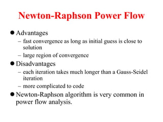
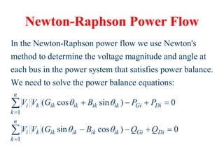
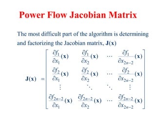
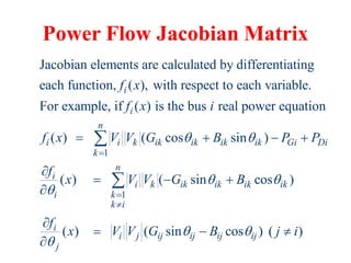
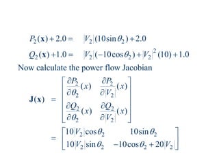
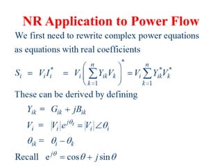
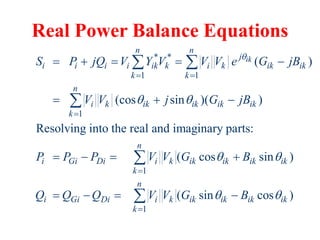
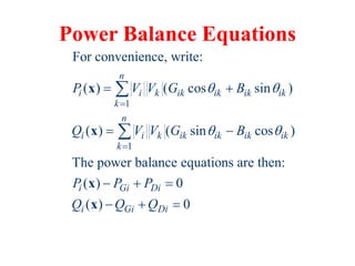
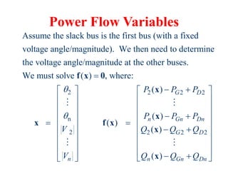
The document discusses the Newton-Raphson power flow method for solving power systems. Some key points: - Newton-Raphson is commonly used for power flow analysis due to its fast convergence when initial guesses are close to the solution and large region of convergence. However, each iteration takes longer than Gauss-Seidel and it is more complicated to code. - It uses Newton's method to determine the voltage magnitude and angle at each bus that satisfies the power balance equations. The power flow Jacobian matrix is calculated by differentiating the real and reactive power balance equations with respect to the voltage variables. 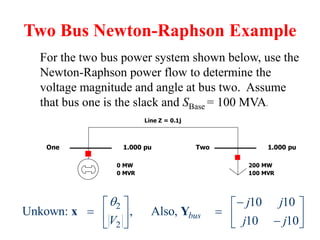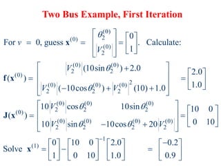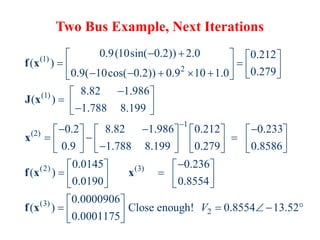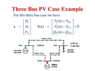- A two-bus example demonstrates setting up and solving the power flow problem using Newton-Raphson

1. Newton-Raphson
Power Flow
Power System Analysis (I)

2. Newton-Raphson Power Flow
 Advantages
– fast convergence as long as initial guess is close to
solution
– large region of convergence
 Disadvantages
– each iteration takes much longer than a Gauss-Seidel
iteration
– more complicated to code
 Newton-Raphson algorithm is very common in
power flow analysis.

3. NR Application to Power Flow

4. Real Power Balance Equations
* *
1 1
1
1
1
( )
(cos sin )( )
Resolving into the real and imaginary parts:
( cos sin )
( sin
ik
n n
j
i i i i ik k i k ik ik
k k
n
i k ik ik ik ik
k
n
i Gi Di i k ik ik ik ik
k
n
i Gi Di i k ik ik
k
S P jQ V Y V V V e G jB
V V j G jB
P P P V V G B
Q Q Q V V G

 
 

 



    
  
   
  
 


 cos )
ik ik
B 


5. Newton-Raphson Power Flow
In the Newton-Raphson power flow we use Newton's
method to determine the voltage magnitude and angle at
each bus in the power system that satisfies power balance.
We need to solve the power balance equ
1
1
ations:
( cos sin ) 0
( sin cos ) 0
n
i k ik ik ik ik Gi Di
k
n
i k ik ik ik ik Gi Di
k
V V G B P P
V V G B Q Q
 
 


   
   



6. Power Balance Equations
1
1
For convenience, write:
( ) ( cos sin )
( ) ( sin cos )
The power balance equations are then:
( ) 0
( ) 0
n
i i k ik ik ik ik
k
n
i i k ik ik ik ik
k
i Gi Di
i Gi Di
P V V G B
Q V V G B
P P P
Q Q Q
 
 


 
 
  
  


x
x
x
x

7. Power Balance Equations
• Note that Pi( ) and Qi( ) mean the functions that
expresses flow from bus i into the system in terms of
voltage magnitudes and angles,
• While PGi, PDi, QGi, QDi mean the generations and
demand at the bus.
• For a system with a slack bus and the rest PQ buses,
power flow problem is to use the power balance
equations to solve for the unknown voltage
magnitudes and angles in terms of the given bus
generations and demands, and then use solution to
calculate the real and reactive injection at the slack
bus.

8. Power Flow Variables
2
n
2
Assume the slack bus is the first bus (with a fixed
voltage angle/magnitude). We then need to determine
the voltage angle/magnitude at the other buses.
We must solve ( ) , where:
n
V
V









f x 0
x
2 2 2
2 2 2
( )
( )
( )
( )
( )
G D
n Gn Dn
G D
n Gn Dn
P P P
P P P
Q Q Q
Q Q Q
 
  
  
  
 
  

   
 
   
   
   
 
 

x
x
f x
x
x

9. N-R Power Flow Solution
(0)
( )
( 1) ( ) ( ) 1 ( )
The power flow is solved using the same procedure
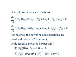
discussed previously for general equations:
For 0; make an initial guess of ,
While ( ) Do
[ ( )] ( )
1
End
v
v v v v
v
v v

 


 
 
x x
f x
x x J x f x

10. Power Flow Jacobian Matrix
1 1 1
1 2 2 2
2 2 2
1 2 2 2
2 2 2 2 2 2
1 2
The most difficult part of the algorithm is determining
and factorizing the Jacobian matrix, ( )
( ) ( ) ( )
( ) ( ) ( )
( )
( ) ( )
n
n
n n n
f f f
x x x
f f f
x x x
f f f
x x x


  
  
  
  
  

  
  
J x
x x x
x x x
J x
x x
2 2
( )
n
 
 
 
 
 
 
 
 
 
 
x

11. Power Flow Jacobian Matrix
1
Jacobian elements are calculated by differentiating
each function, ( ), with respect to each variable.
For example, if ( ) is the bus real power equation
( ) ( cos sin )
i
i
n
i i k ik ik ik ik Gi
k
f x
f x i
f x V V G B P P
 

   

1
( ) ( sin cos )
( ) ( sin cos ) ( )
Di
n
i
i k ik ik ik ik
i k
k i
i
i j ij ij ij ij
j
f
x V V G B
f
x V V G B j i
 

 




  


  



12. Two Bus Newton-Raphson Example
Line Z = 0.1j
One Two
1.000 pu 1.000 pu
200 MW
100 MVR
0 MW
0 MVR
For the two bus power system shown below, use the
Newton-Raphson power flow to determine the
voltage magnitude and angle at bus two. Assume
that bus one is the slack and SBase = 100 MVA.
2
2
10 10
Unkown: , Also,
10 10
bus
j j
V j j
 
   
 
   

 
 
x Y

13. 1
1
General power balance equations:
( cos sin ) 0
( sin cos ) 0
For bus two, the power balance equations are
(load real power is 2.0 per unit,
while react
n
i k ik ik ik ik Gi Di
k
n
i k ik ik ik ik Gi Di
k
V V G B P P
V V G B Q Q
 
 


   
   


2 1 2
2
2 1 2 2
ive power is 1.0 per unit):
(10sin ) 2.0 0
( 10cos ) (10) 1.0 0
V V
V V V


 
   

14. 2 2 2
2
2 2 2 2
2 2
2 2
2 2
2 2
2 2 2
2 2 2 2
( ) 2.0 (10sin ) 2.0
( ) 1.0 ( 10cos ) (10) 1.0
Now calculate the power flow Jacobian
( ) ( )
( )
( ) ( )
10 cos 10sin
10 sin 10cos 20
P V
Q V V
P P
x x
V
Q Q
x x
V
V
V V




 
 
  
    
 
 
 
 
 

 
 
 
 
 
 
  
 
 
x
x
J x

15. Two Bus Example, First Iteration
(0)
2
(0)
(0)
2
(0) (0)
2 2
(0)
2
(0) (0) (0)
2 2 2
(0) (0) (0)
2 2 2
(0)
(0) (0)
2 2
0
For 0, guess . Calculate:
1
(10sin ) 2.0 2.0
( )
1.0
( 10cos ) (10) 1.0
10 cos 10sin
( )
10 sin 10cos
v
V
V
V V
V
V



 

   
  
   
 
 
 
 

 
 
   
   
  
 


x
f x
J x
(0) (0)
2 2
1
(1)
10 0
0 10
20
0 10 0 2.0 0.2
Solve
1 0 10 1.0 0.9
V


 
 
    
   

 

       
  
       
       
x

16. Two Bus Example, Next Iterations
(1)
2
(1)
1
(2)
0.9(10sin( 0.2)) 2.0 0.212
( )
0.279
0.9( 10cos( 0.2)) 0.9 10 1.0
8.82 1.986
( )
1.788 8.199
0.2 8.82 1.986 0.212 0.233
0.9 1.788 8.199 0.279 0.8586
(

 
   
 
   
      
 

 
  

 
  
       
  
       

       
f x
J x
x
f (2) (3)
(3)
2
0.0145 0.236
)
0.0190 0.8554
0.0000906
( ) Close enough! 0.8554 13.52
0.0001175
V

   
 
   
   
 
    
 
 
x x
f x

17. PV Buses
Since the voltage magnitude at PV buses is fixed
there is no need to explicitly include these voltages
in x nor explicitly include the reactive power
balance equations at the PV buses:
– the reactive power output of the generator varies to
maintain the fixed terminal voltage (within limits), so
we can just use the solved voltages and angles to
calculate the reactive power production to be whatever
is needed to satisfy reactive power balance.
– An alternative is to keep the reactive power balance
equation explicit but also write an explicit voltage
constraint for the generator bus:
|Vi | – Vi setpoint = 0

18. Three Bus PV Case Example
Line Z = 0.1j
Line Z = 0.1j Line Z = 0.1j
One Two
1.000 pu
0.941 pu
200 MW
100 MVR
170.0 MW
68.2 MVR
-7.469 Deg
Three 1.000 pu
30 MW
63 MVR
2 2 2
3 3 3
2 2 2
For this three bus case we have
( )
( ) ( ) 0
( )
D
G
D
P P
P P
V Q Q



   
   
   
   

 
   
 
x
x f x x
x

19. PV Buses
• With Newton-Raphson, PV buses means that there
are less unknown variables we need to calculate
explicitly and less equations we need to satisfy
explicitly.
• Reactive power balance is satisfied implicitly by
choosing reactive power production to be whatever
is needed, once we have a solved case (like real and
reactive power at the slack bus).
• Contrast to Gauss iterations where PV buses
complicated the algorithm.