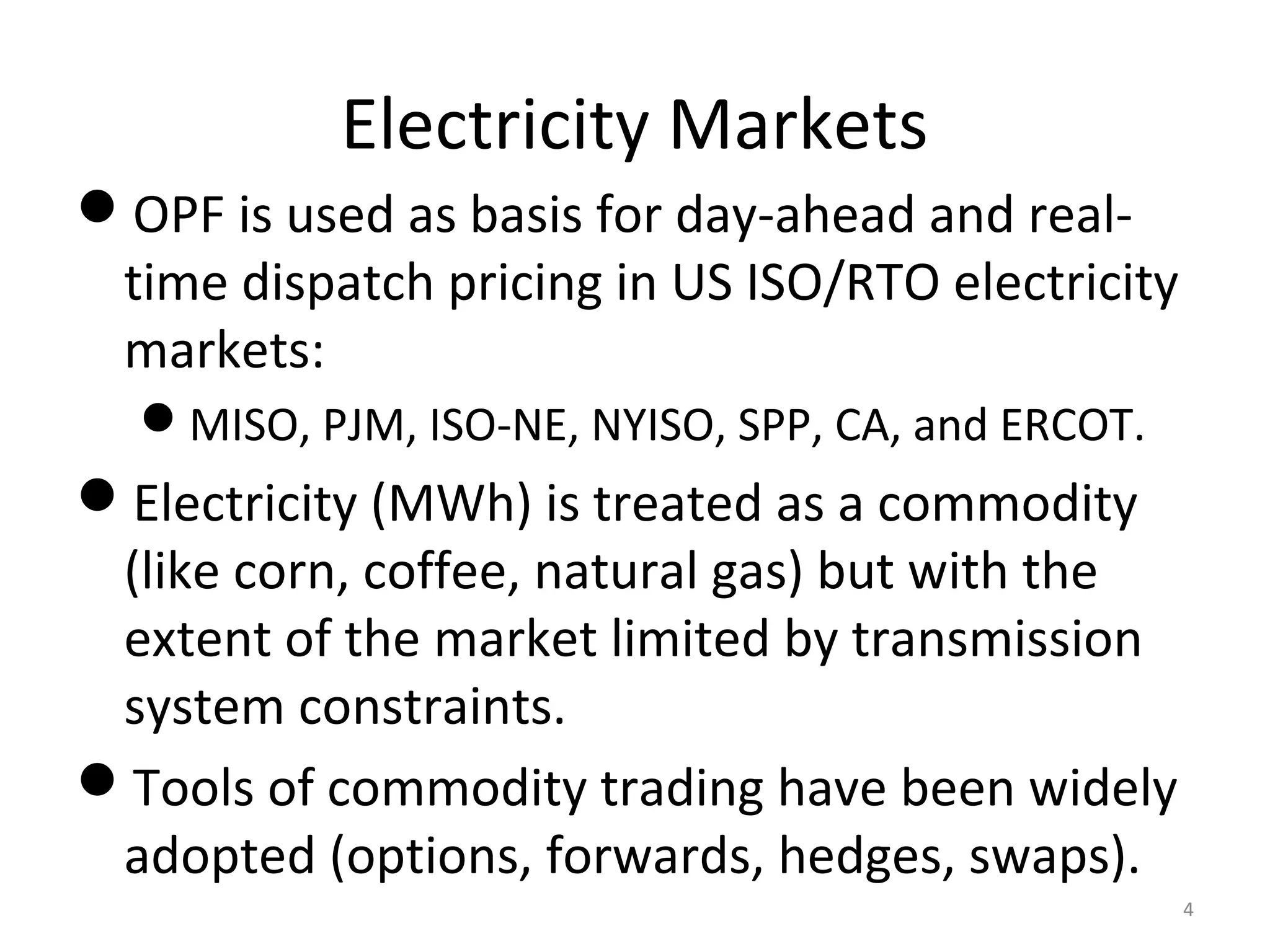
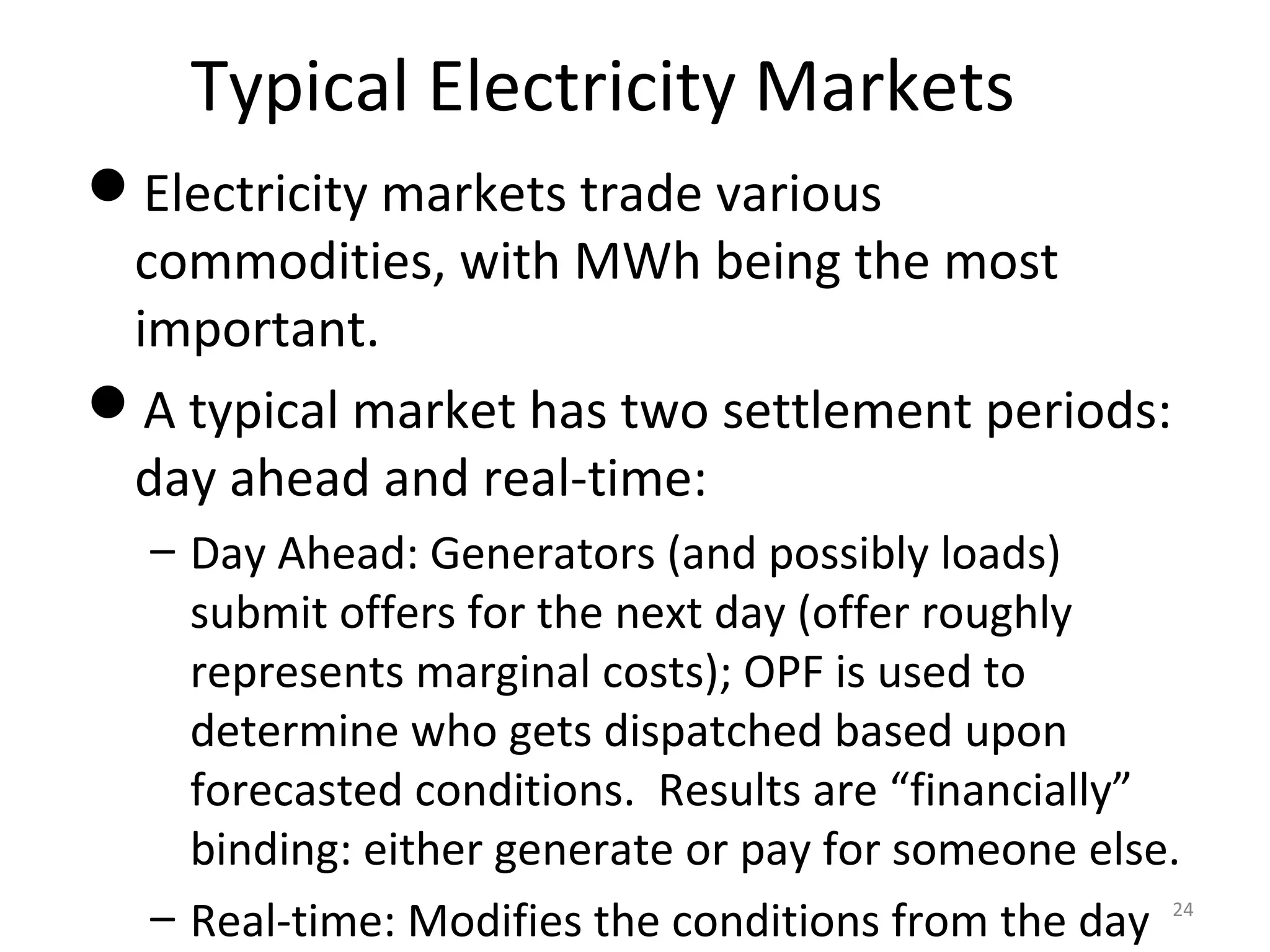
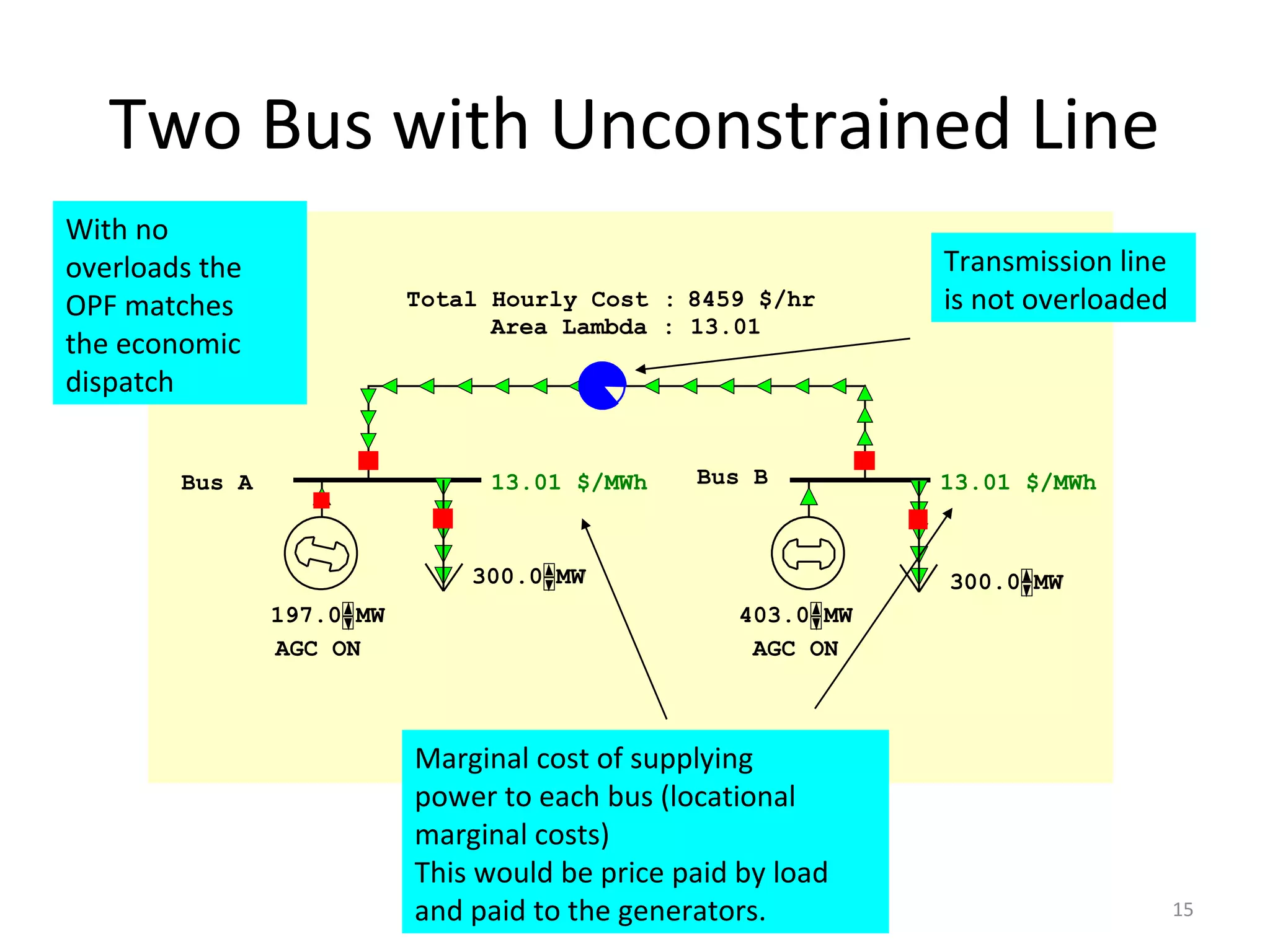
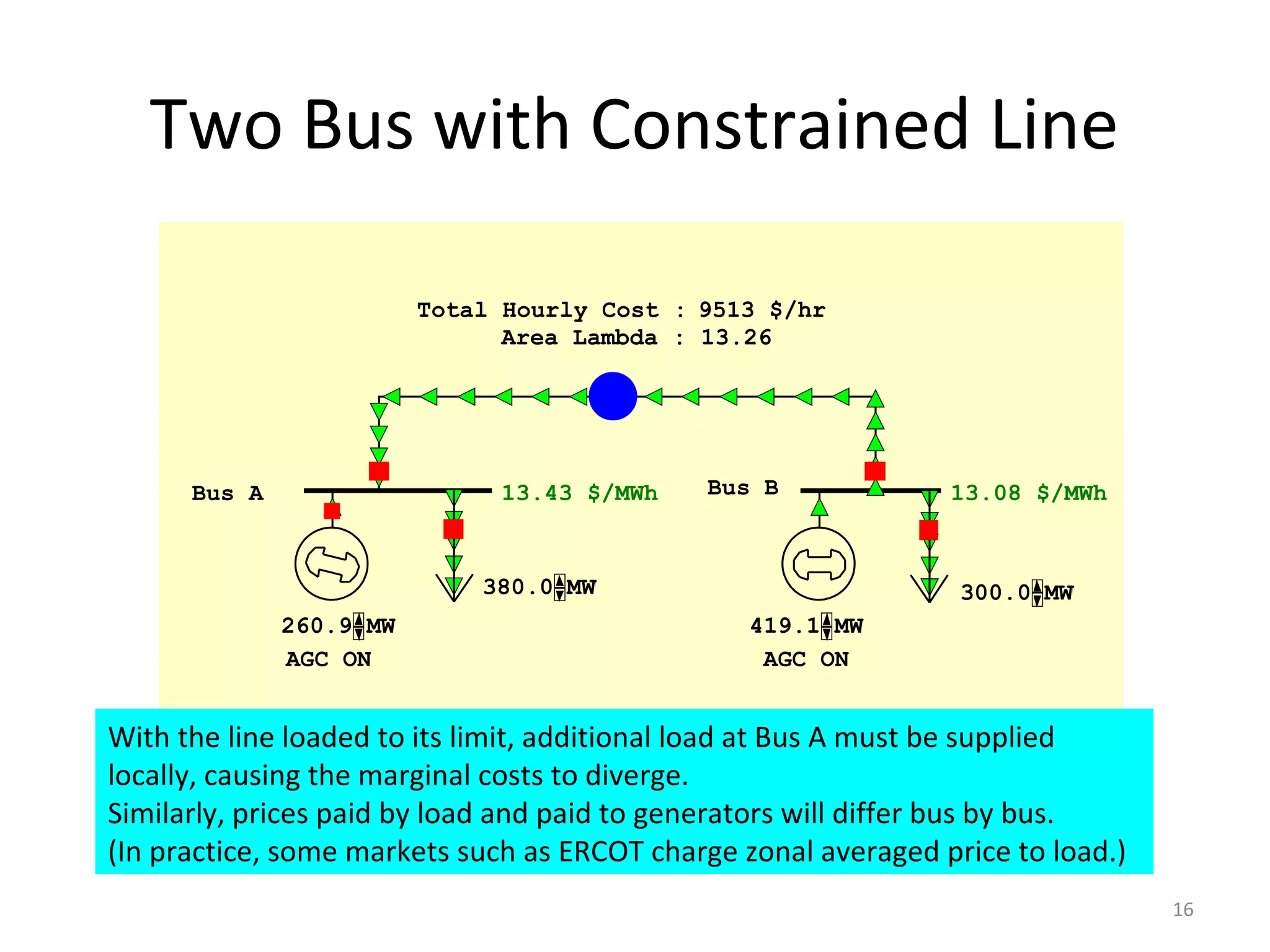
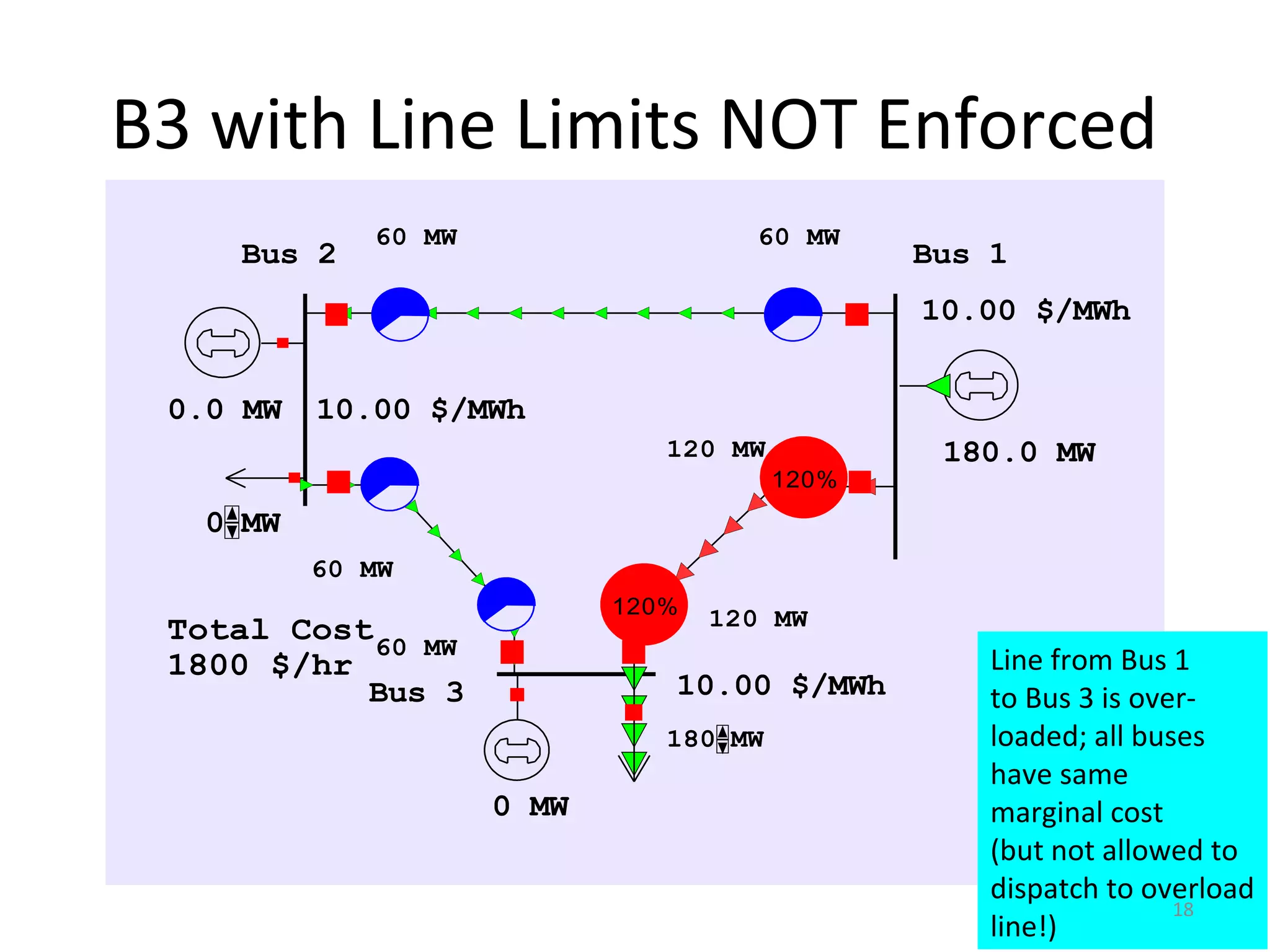
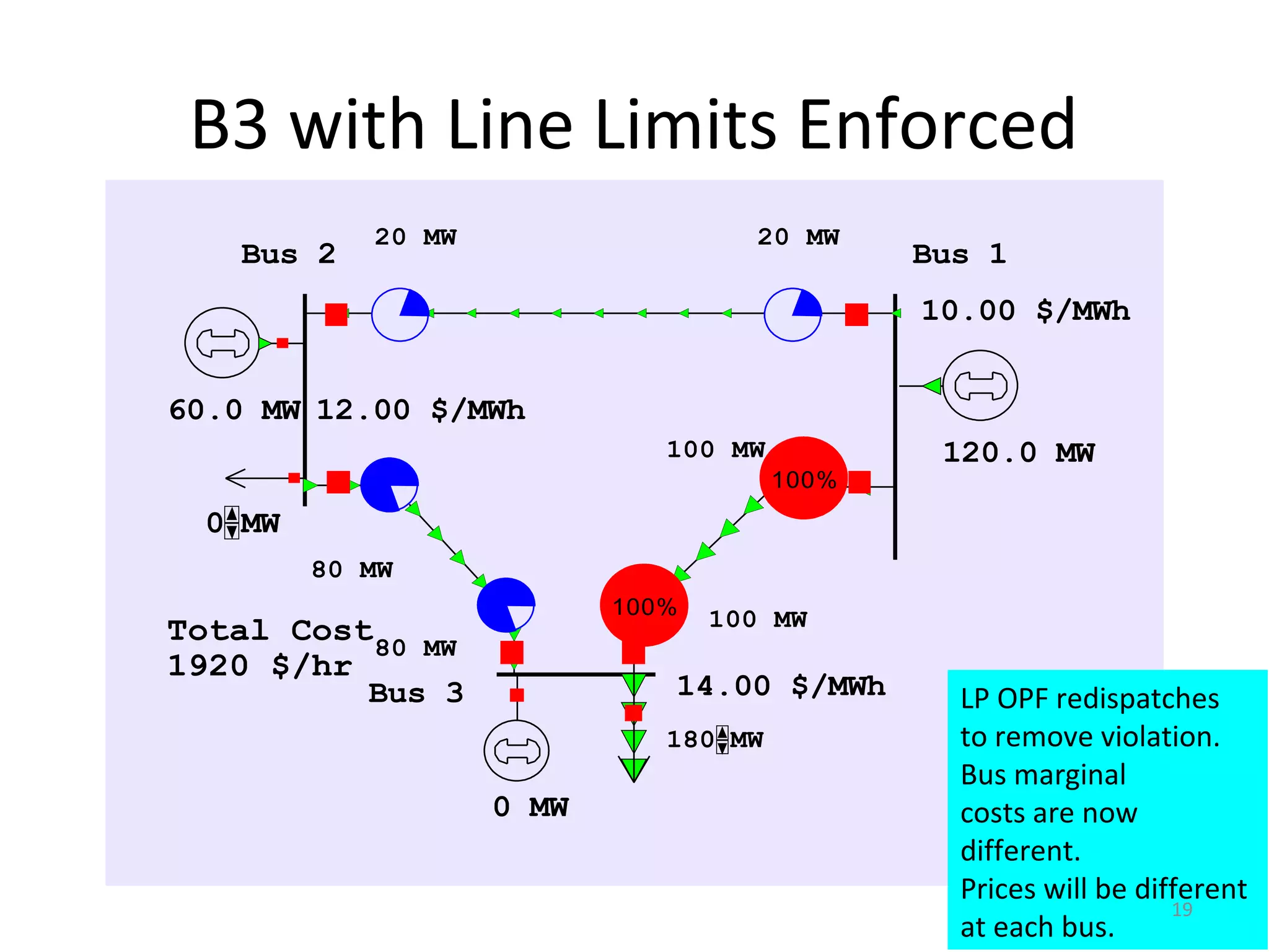
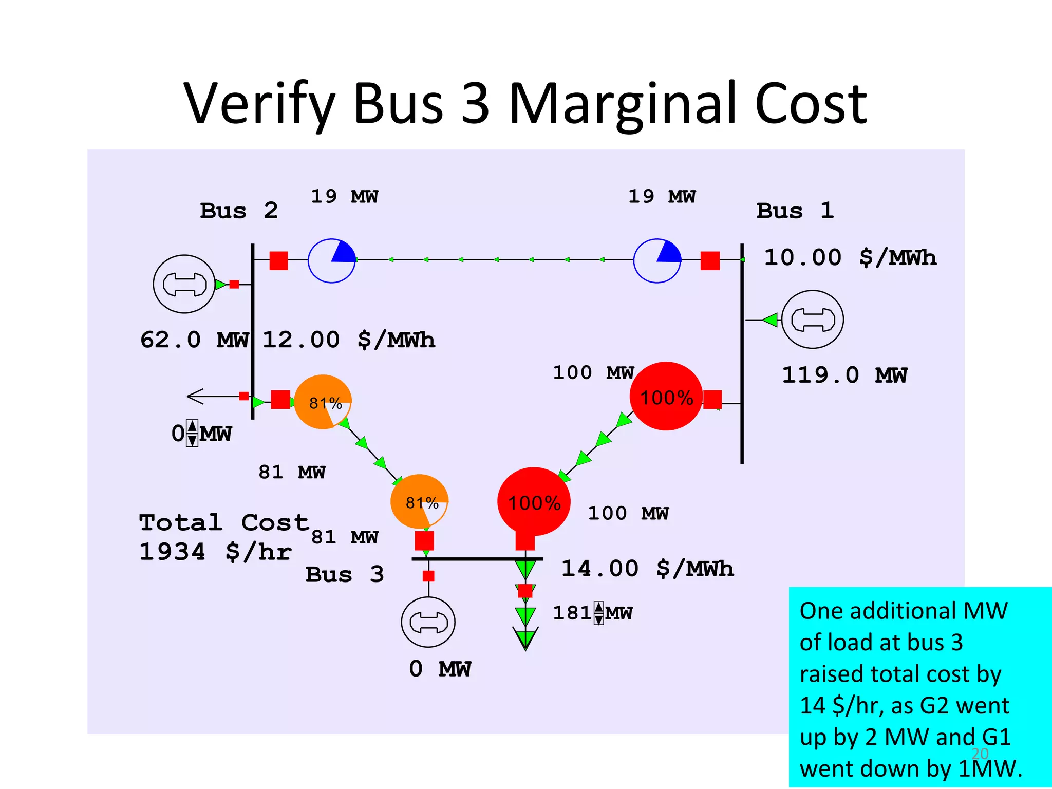
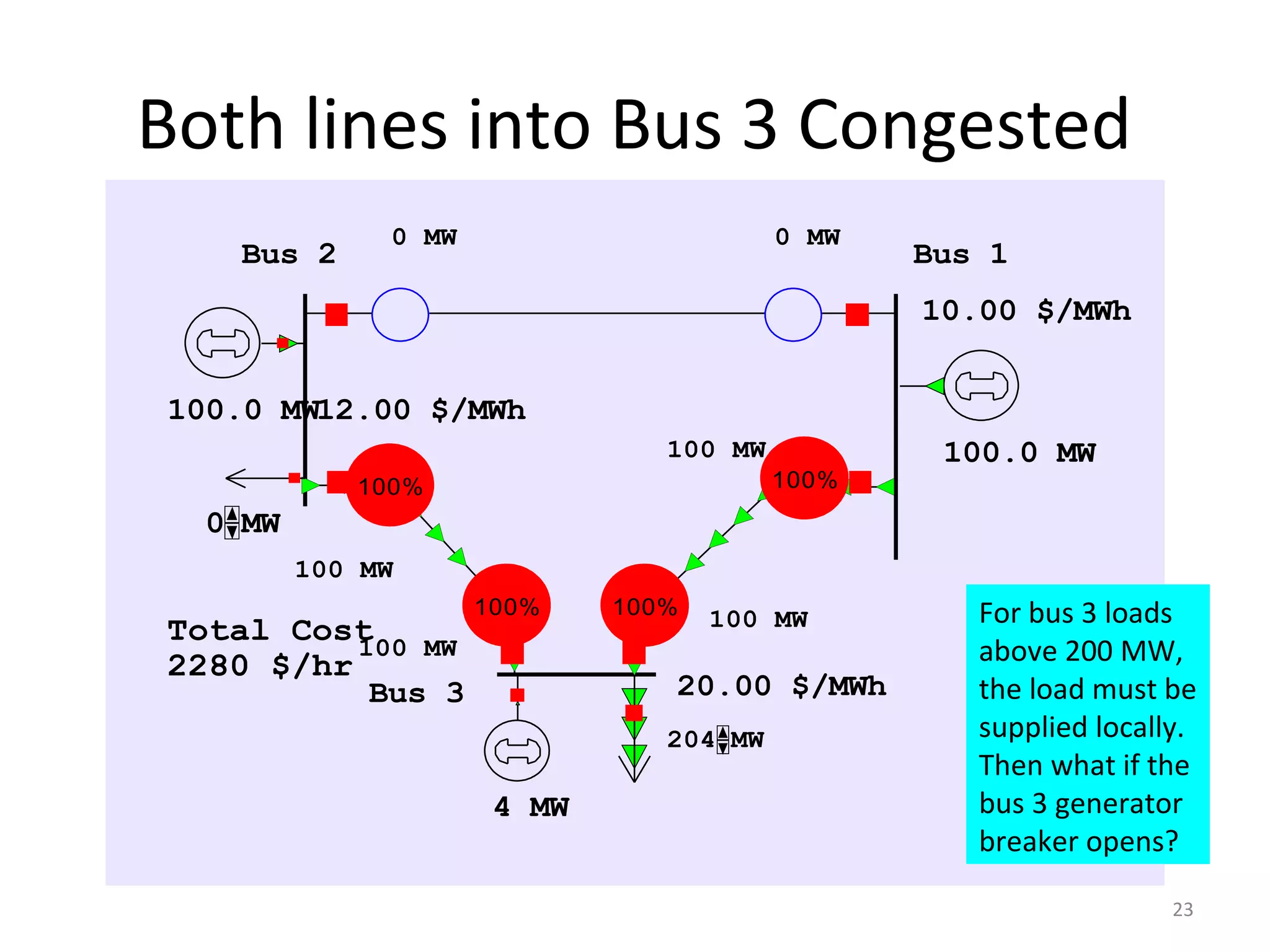
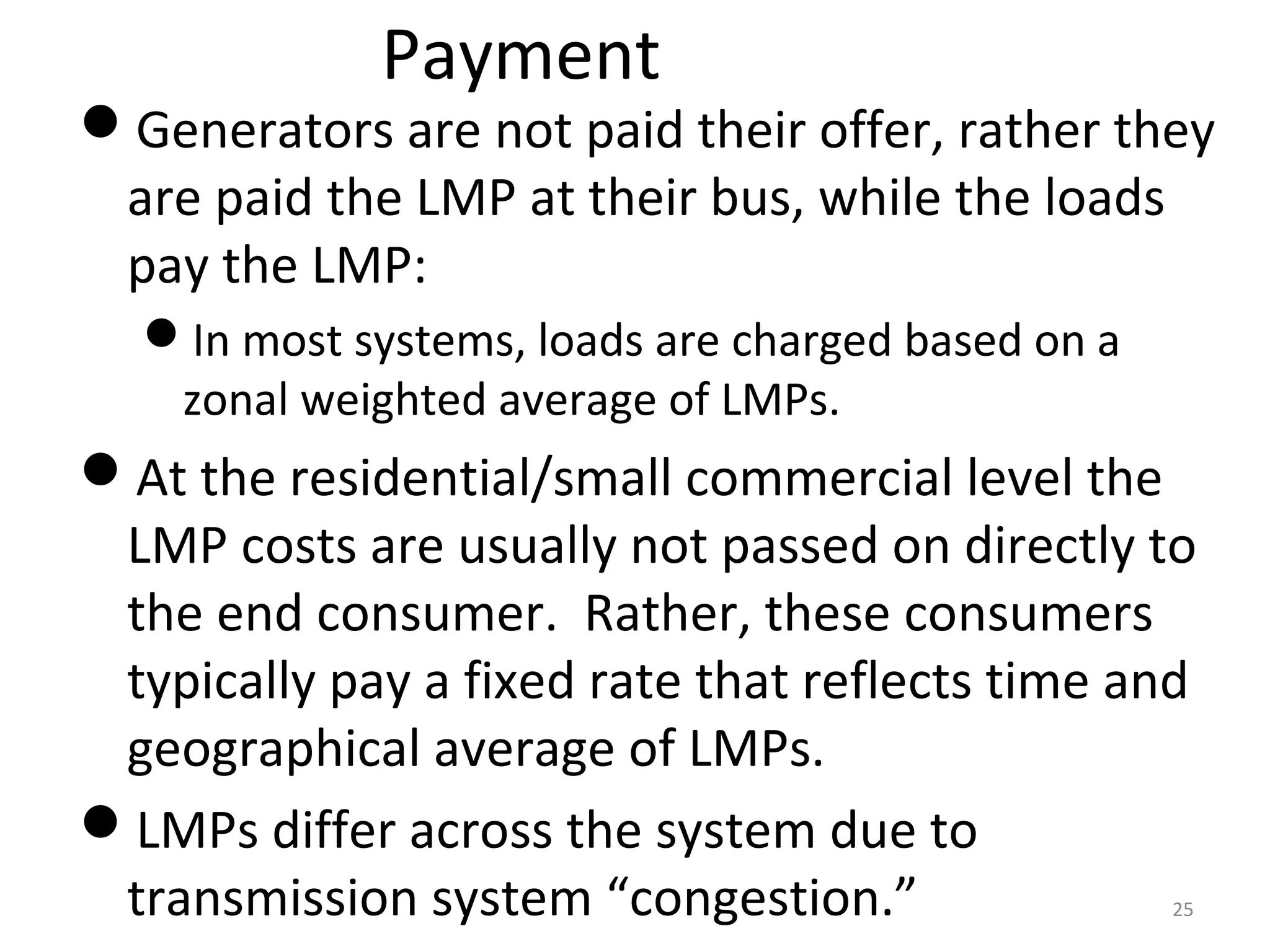
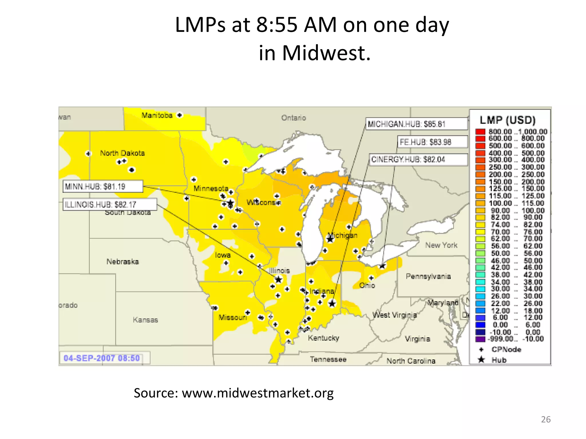
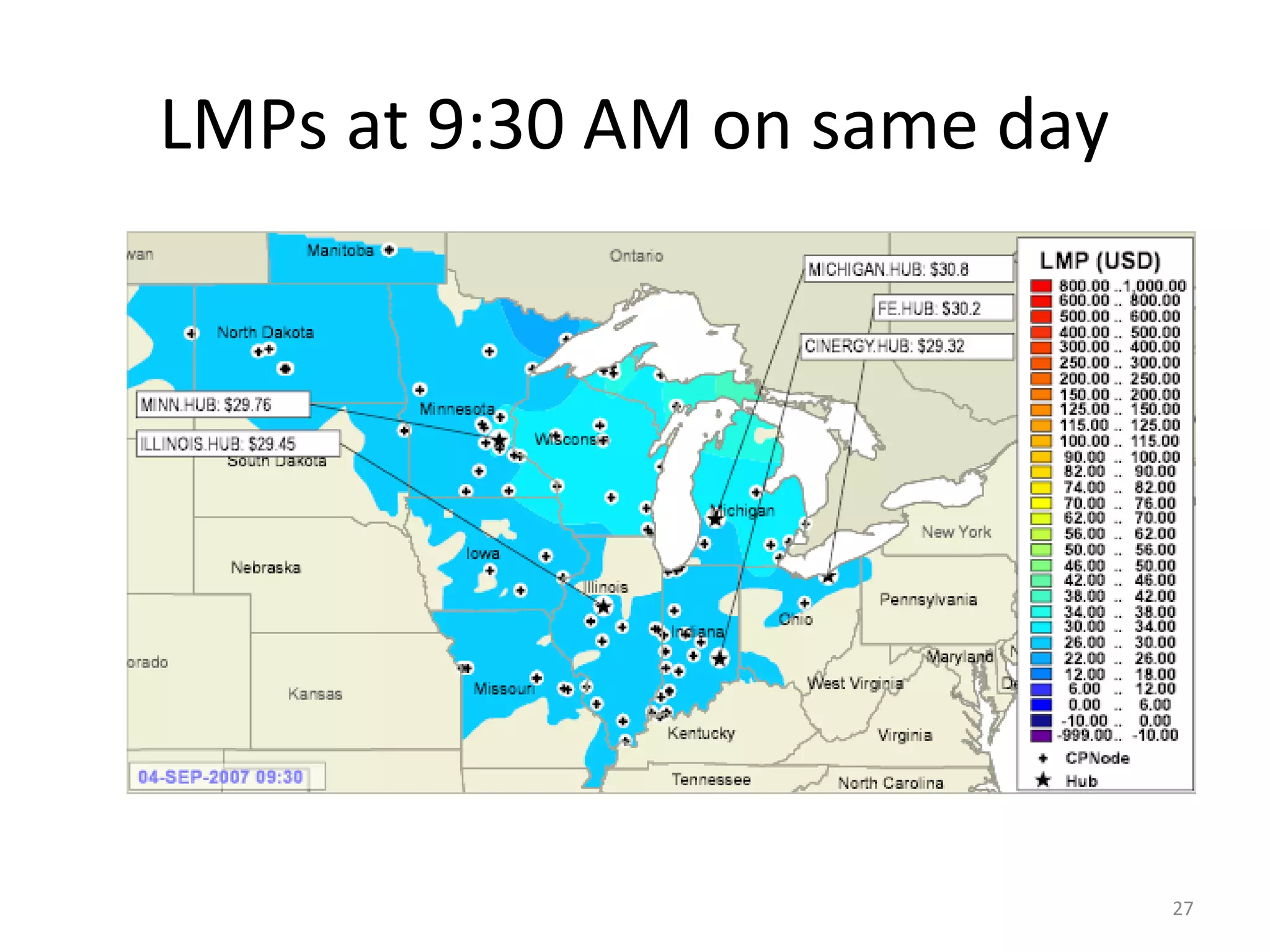
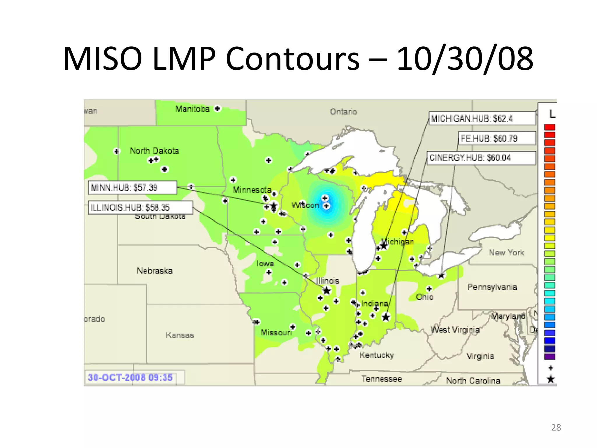
This document discusses optimal power flow (OPF) and locational marginal pricing (LMP) in electricity markets. It provides the following key points: 1) OPF is used by Independent System Operators to determine day-ahead and real-time dispatch pricing based on generators' marginal costs while accounting for transmission constraints. 2) LMP indicates the marginal cost of supplying additional electricity to a bus. It differs across buses due to transmission constraints identified through OPF. 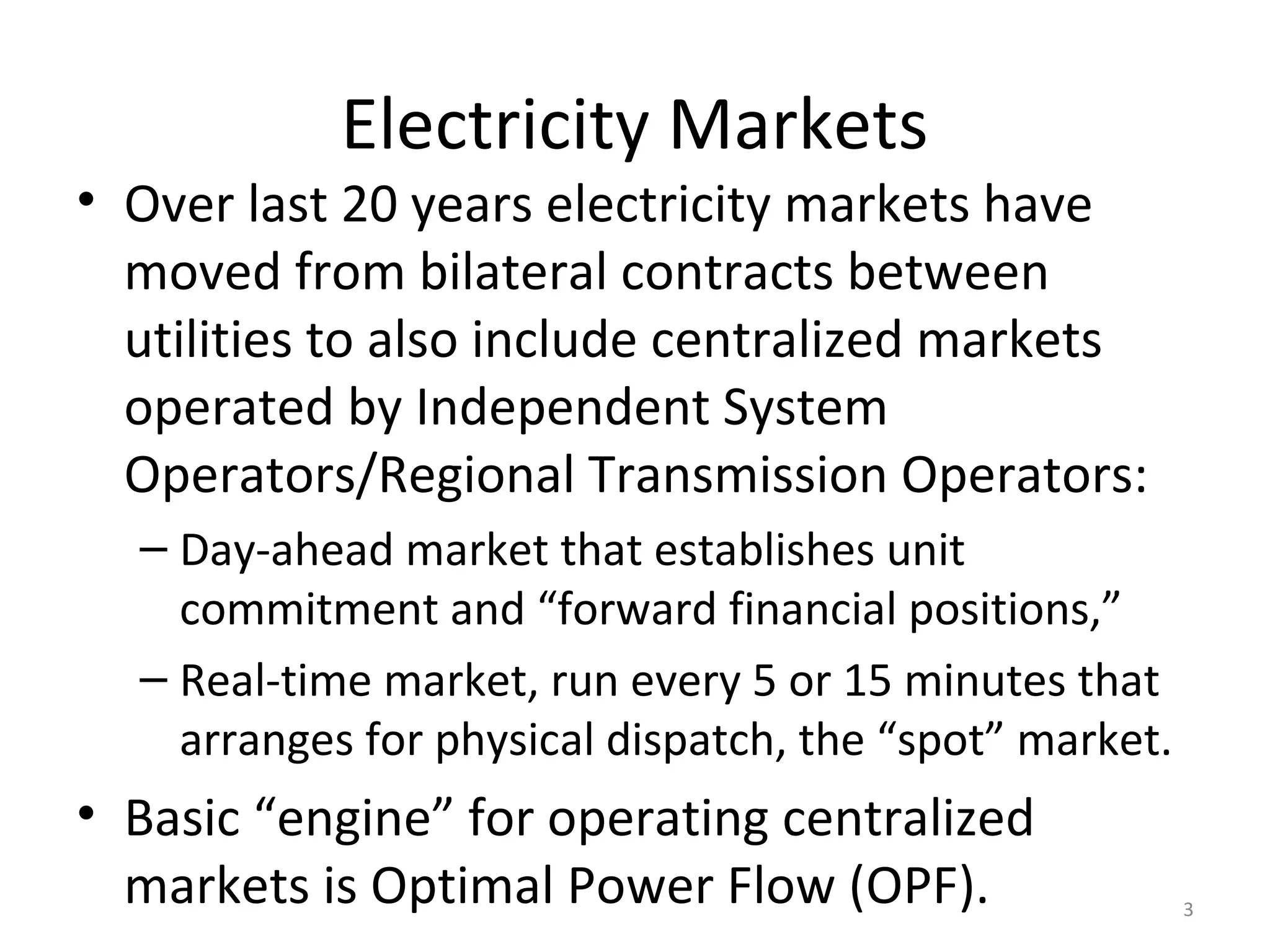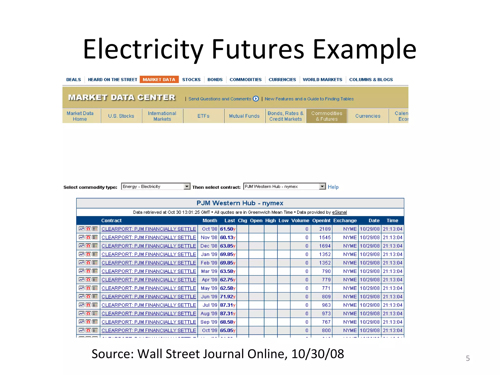3) Electricity markets have moved from bilateral contracts to centralized day-ahead and real-time markets operated by ISOs using OPF and LMP to function like commodity markets while respecting transmission limits.

1. EE 369
POWER SYSTEM ANALYSIS
Lecture 17
Optimal Power Flow, LMPs
Tom Overbye and Ross Baldick
1

2. Announcements
Read Chapter 7.
Homework 12 is 6.59, 6.61, 12.19, 12.22,
12.24, 12.26, 12.28, 7.1, 7.3, 7.4, 7.5, 7.6,
7.9, 7.12, 7.16; due Thursday, 12/3.
2

3. Electricity Markets
• Over last 20 years electricity markets have
moved from bilateral contracts between
utilities to also include centralized markets
operated by Independent System
Operators/Regional Transmission Operators:
– Day-ahead market that establishes unit
commitment and “forward financial positions,”
– Real-time market, run every 5 or 15 minutes that
arranges for physical dispatch, the “spot” market.
• Basic “engine” for operating centralized
markets is Optimal Power Flow (OPF). 3

4. Electricity Markets
OPF is used as basis for day-ahead and real-
time dispatch pricing in US ISO/RTO electricity
markets:
MISO, PJM, ISO-NE, NYISO, SPP, CA, and ERCOT.
Electricity (MWh) is treated as a commodity
(like corn, coffee, natural gas) but with the
extent of the market limited by transmission
system constraints.
Tools of commodity trading have been widely
adopted (options, forwards, hedges, swaps).
4

5. Electricity Futures Example
Source: Wall Street Journal Online, 10/30/08 5

6. “Ideal” Power Market
Ideal power market is analogous to a lake.
Generators supply energy to lake and loads
remove energy.
Ideal power market has no transmission
constraints
Single marginal cost associated with enforcing
constraint that supply = demand
– buy from the least cost unit that is not at a limit
– this price is the marginal cost.
This solution is identical to the economic
dispatch problem solution. 6

7. Two Bus ED Example
Total Hourly Cost :
Bus A Bus B
300.0 MWMW
199.6 MWMW 400.4 MWMW
300.0 MWMW
8459 $/hr
Area Lambda : 13.02
AGC ON AGC ON
7

8. Market Marginal (Incremental)
Cost
0 175 350 525 700
Generator Power (MW)
12.00
13.00
14.00
15.00
16.00
Below are some graphs associated with this two bus system. The graph on left
shows the marginal cost for each of the generators. The graph on the right
shows the system supply curve, assuming the system is optimally dispatched.
Current generator operating point
0 350 700 1050 1400
Total Area Generation (MW)
12.00
13.00
14.00
15.00
16.00
8

9. Real Power Markets
Different operating regions impose
constraints – may limit ability to achieve
economic dispatch “globally.”
Transmission system imposes constraints on
the market:
Marginal costs differ at different buses.
Optimal dispatch solution requires solution by
an optimal power flow
Charging for energy based on marginal costs
at different buses is called “locational
marginal pricing” (LMP) or “nodal” pricing. 9

10. Pricing Electricity
LMP indicates the additional cost to supply an
additional amount of electricity to bus.
All North American ISO/RTO electricicity markets
price wholesale energy at LMP.
If there were no transmission limitations then the
LMPs would be the same at all buses:
Equal to value of lambda from economic dispatch.
Transmission constraints result in differing LMPs at
buses.
Determination of LMPs requires the solution of an
“Optimal Power Flow” (OPF).
10

11. Optimal Power Flow (OPF)
OPF functionally combines the power flow
with economic dispatch.
Minimize cost function, such as operating
cost, taking into account realistic equality and
inequality constraints.
Equality constraints:
– bus real and reactive power balance
– generator voltage setpoints
– area MW interchange
11

12. OPF, cont’d
Inequality constraints:
– transmission line/transformer/interface flow
limits
– generator MW limits
– generator reactive power capability curves
– bus voltage magnitudes (not yet implemented in
Simulator OPF)
Available Controls:
– generator MW outputs
– transformer taps and phase angles 12

13. OPF Solution Methods
Non-linear approach using Newton’s method:
– handles marginal losses well, but is relatively slow
and has problems determining binding constraints
Linear Programming (LP):
– fast and efficient in determining binding
constraints, but can have difficulty with marginal
losses.
– used in PowerWorld Simulator
13

14. LP OPF Solution Method
Solution iterates between:
– solving a full ac power flow solution
enforces real/reactive power balance at each bus
enforces generator reactive limits
system controls are assumed fixed
takes into account non-linearities
– solving an LP
changes system controls to enforce linearized
constraints while minimizing cost
14

15. Two Bus with Unconstrained Line
Total Hourly Cost :
Bus A Bus B
300.0 MWMW
197.0 MWMW 403.0 MWMW
300.0 MWMW
8459 $/hr
Area Lambda : 13.01
AGC ON AGC ON
13.01 $/MWh 13.01 $/MWh
Transmission line
is not overloaded
With no
overloads the
OPF matches
the economic
dispatch
Marginal cost of supplying
power to each bus (locational
marginal costs)
This would be price paid by load
and paid to the generators. 15

16. Two Bus with Constrained Line
Total Hourly Cost :
Bus A Bus B
380.0 MWMW
260.9 MWMW 419.1 MWMW
300.0 MWMW
9513 $/hr
Area Lambda : 13.26
AGC ON AGC ON
13.43 $/MWh 13.08 $/MWh
With the line loaded to its limit, additional load at Bus A must be supplied
locally, causing the marginal costs to diverge.
Similarly, prices paid by load and paid to generators will differ bus by bus.
(In practice, some markets such as ERCOT charge zonal averaged price to load.)
16

17. Three Bus (B3) Example
Consider a three bus case (bus 1 is system
slack), with all buses connected through 0.1
pu reactance lines, each with a 100 MVA limit.
Let the generator marginal costs be:
– Bus 1: 10 $ / MWhr; Range = 0 to 400 MW,
– Bus 2: 12 $ / MWhr; Range = 0 to 400 MW,
– Bus 3: 20 $ / MWhr; Range = 0 to 400 MW,
Assume a single 180 MW load at bus 2.
17

18. Bus 2 Bus 1
Bus 3
Total Cost
0.0 MW
0 MW
180 MW
10.00 $/MWh
60 MW 60 MW
60 MW
60 MW
120 MW
120 MW
10.00 $/MWh
10.00 $/MWh
180.0 MW
0 MW
1800 $/hr
120%
120%
B3 with Line Limits NOT Enforced
Line from Bus 1
to Bus 3 is over-
loaded; all buses
have same
marginal cost
(but not allowed to
dispatch to overload
line!)
18

19. B3 with Line Limits Enforced
Bus 2 Bus 1
Bus 3
Total Cost
60.0 MW
0 MW
180 MW
12.00 $/MWh
20 MW 20 MW
80 MW
80 MW
100 MW
100 MW
10.00 $/MWh
14.00 $/MWh
120.0 MW
0 MW
1920 $/hr
100%
100%
LP OPF redispatches
to remove violation.
Bus marginal
costs are now
different.
Prices will be different
at each bus.
19

20. Bus 2 Bus 1
Bus 3
Total Cost
62.0 MW
0 MW
181 MW
12.00 $/MWh
19 MW 19 MW
81 MW
81 MW
100 MW
100 MW
10.00 $/MWh
14.00 $/MWh
119.0 MW
0 MW
1934 $/hr
81%
81%
100%
100%
Verify Bus 3 Marginal Cost
One additional MW
of load at bus 3
raised total cost by
14 $/hr, as G2 went
up by 2 MW and G1
went down by 1MW.
20

21. Why is bus 3 LMP = $14 /MWh ?
All lines have equal impedance. Power flow
in a simple network distributes inversely to
impedance of path.
– For bus 1 to supply 1 MW to bus 3, 2/3 MW would
take direct path from 1 to 3, while 1/3 MW would
“loop around” from 1 to 2 to 3.
– Likewise, for bus 2 to supply 1 MW to bus 3,
2/3MW would go from 2 to 3, while 1/3 MW
would go from 2 to 1to 3.
21

22. Why is bus 3 LMP $ 14 / MWh,
cont’d
With the line from 1 to 3 limited, no
additional power flows are allowed on it.
To supply 1 more MW to bus 3 we need:
– Extra production of 1MW: Pg1 + Pg2 = 1 MW
– No more flow on line 1 to 3: 2/3 Pg1 + 1/3 Pg2 = 0;
 Solving requires we increase Pg2 by 2 MW and
decrease Pg1 by 1 MW – for a net increase of
$14/h for the 1 MW increase.
That is, the marginal cost of delivering power22

23. Both lines into Bus 3 Congested
Bus 2 Bus 1
Bus 3
Total Cost
100.0 MW
4 MW
204 MW
12.00 $/MWh
0 MW 0 MW
100 MW
100 MW
100 MW
100 MW
10.00 $/MWh
20.00 $/MWh
100.0 MW
0 MW
2280 $/hr
100% 100%
100% 100% For bus 3 loads
above 200 MW,
the load must be
supplied locally.
Then what if the
bus 3 generator
breaker opens?
23

24. Typical Electricity Markets
Electricity markets trade various
commodities, with MWh being the most
important.
A typical market has two settlement periods:
day ahead and real-time:
– Day Ahead: Generators (and possibly loads)
submit offers for the next day (offer roughly
represents marginal costs); OPF is used to
determine who gets dispatched based upon
forecasted conditions. Results are “financially”
binding: either generate or pay for someone else.
– Real-time: Modifies the conditions from the day 24

25. Payment
Generators are not paid their offer, rather they
are paid the LMP at their bus, while the loads
pay the LMP:
In most systems, loads are charged based on a
zonal weighted average of LMPs.
At the residential/small commercial level the
LMP costs are usually not passed on directly to
the end consumer. Rather, these consumers
typically pay a fixed rate that reflects time and
geographical average of LMPs.
LMPs differ across the system due to
transmission system “congestion.” 25

26. LMPs at 8:55 AM on one day
in Midwest.
Source: www.midwestmarket.org
26

27. LMPs at 9:30 AM on same day
27

28. MISO LMP Contours – 10/30/08
28

29. Limiting Carbon Dioxide Emissions
• There is growing concern about the need to
limit carbon dioxide emissions.
• The two main approaches are 1) a carbon tax,
or 2) a cap-and-trade system (emissions
trading)
• The tax approach involves setting a price and
emitter of CO2 pays based upon how much CO2 is
emitted.
• A cap-and-trade system limits emissions by
requiring permits (allowances) to emit CO2. The
government sets the number of allowances,
allocates them initially, and then private markets set
their prices and allow trade.
29