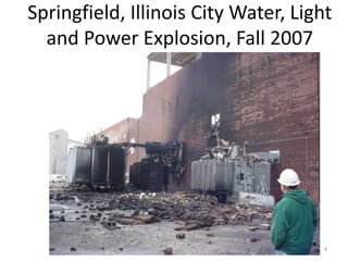
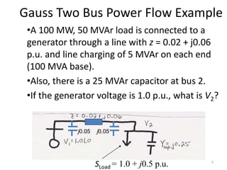
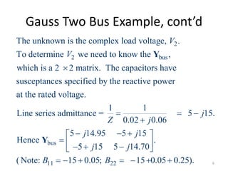
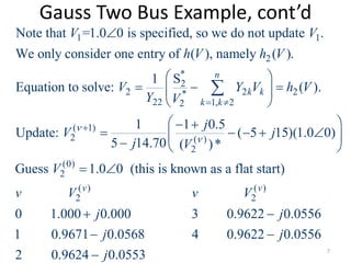
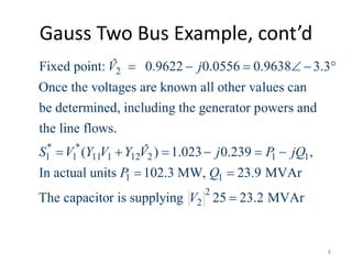
This document provides an overview of load flow analysis and power flow solution techniques, specifically the Gauss-Seidel and Newton-Raphson methods. It begins with an example Gauss-Seidel power flow calculation for a two bus system. It then discusses the inclusion of PV generator buses in the Gauss-Seidel iteration and accelerated Gauss-Seidel convergence. The document concludes by introducing the Newton-Raphson power flow algorithm and comparing the advantages and disadvantages of Gauss-Seidel versus Newton-Raphson.

1. Load Flow Analysis
Part- I
Prepared by – A. L. Jamadar
1

2. Wind Blade Failure
Photo source: Peoria Journal Star
Several years ago, a 140 foot,
6.5 ton blade broke off from a
Suzlon Energy wind turbine.
The wind turbine is located
in Illinois. Suzlon Energy is
one of the world’s largest
wind turbine manufacturers;
its shares fell 39% following
the accident. No one was hurt
and wind turbines failures
are extremely rare events.
(Vestas and Siemens turbines
have also failed.) 2

3. Thermal Plants Can Fail As Well: Another Illinois
Failure, Fall 2007
3

4. Springfield, Illinois City Water, Light
and Power Explosion, Fall 2007
4

5. Gauss Two Bus Power Flow Example
•A 100 MW, 50 MVAr load is connected to a
generator through a line with z = 0.02 + j0.06
p.u. and line charging of 5 MVAr on each end
(100 MVA base).
•Also, there is a 25 MVAr capacitor at bus 2.
•If the generator voltage is 1.0 p.u., what is V2?
SLoad = 1.0 + j0.5 p.u. 5
j0.05 j0.05

6. Gauss Two Bus Example, cont’d
2
2 bus
The unknown is the complex load voltage, .
To determine we need to know the ,
which is a 2 2 matrix. The capacitors have
susceptances specified by the reactive power
at the rated voltage.
Line
V
V

Y
bus
11 22
1 1
series admittance = 5 15.
0.02 0.06
5 14.95 5 15
Hence .
5 15 5 14.70
( Note: 15 0.05; 15 0.05 0.25).
j
Z j
j j
j j
B B
  

   
     
      
Y
6

7. Gauss Two Bus Example, cont’d
1 1
2
*
2
2 2 2*
22 1, 22
( 1)
2
2
Note that =1.0 0 is specified, so we do not update .
We only consider one entry of ( ), namely ( ).
1 S
Equation to solve: ( ).
1 1 0.5
Update:
5 14.70 (
n
k k
k k
V V
h V h V
V Y V h V
Y V
j
V
j V

 


 
   
 
 



( )
(0)
2
( ) ( )
2 2
( 5 15)(1.0 0)
)*
Guess 1.0 0 (this is known as a flat start)
0 1.000 0.000 3 0.9622 0.0556
1 0.9671 0.0568 4 0.9622 0.0556
2 0.9624 0.0553
v v
j
V
v V v V
j j
j j
j

 
    
 
 
 
 
 7

8. Gauss Two Bus Example, cont’d
2
* *
1 1 11 1 12 2 1 1
ˆFixed point: 0.9622 0.0556 0.9638 3.3
Once the voltages are known all other values can
be determined, including the generator powers and
the line flows.
ˆ( ) 1.023 0.239 ,
V j
S V Y V Y V j P jQ
     
     
1 1
2
2
In actual units 102.3 MW, 23.9 MVAr
The capacitor is supplying 25 23.2 MVAr
P Q
V
 

8

9. Slack Bus
In this example we specified S2 and V1 and then
solved for S1 and V2.
We can not arbitrarily specify S at all buses
because total generation must equal total load +
total losses: “real and reactive power balance.”
In addition, we also need an angle reference bus.
To solve these problems we define one bus as
the “slack” bus to deal with both issues:
Slack bus has a fixed voltage magnitude and angle,
and a varying real/reactive power injection to satisfy
overall real and reactive power balance.
In the example, this was bus 1. 9

10. Gauss for Systems with Many Buses
*
( 1) ( )
( )*
1,
( ) ( ) ( )
1 2
( 1)
With multiple bus systems we could calculate
new values of the voltages as follows:
S1
( , ,..., )
But after we've determined , it is
i
i
n
v vi
i ik kv
ii k k i
v v v
i n
v
i
V
V Y V
Y V
h V V V
V

 

 
  
 
 


( )
a better estimate
of the voltage at bus than , so it makes sense to use
this new value. Using the latest values is known as the
Gauss-Seidel iteration.
v
ii V
10

11. Gauss-Seidel Iteration
( 1) ( ) ( ) ( )
2 12 2 3
( 1) ( 1) ( ) ( )
3 13 2 3
( 1) ( 1) ( 1) ( ) ( )
4 14 2 3 4
( 1) ( 1) (
1 2 3
Immediately use the new voltage estimates:
( , , , , ) (bus 1 is slack),
( , , , , )
( , , , , )
( , ,
v v v v
n
v v v v
n
v v v v v
n
v v v
n n
V h V V V V
V h V V V V
V h V V V V V
V h V V V

 
  
 
 
 
 

M
1) ( 1) ( )
4, , )
Gauss-Seidel usually works better than the Gauss, and
is actually easier to implement.
Gauss-Seidel is used in practice instead of Gauss.
v v
nV V 

11

12. Three Types of Power Flow Buses
There are three main types of buses:
– Load (PQ), at which P and Q are fixed; goal is to
solve for unknown voltage magnitude and angle at
the bus (some generators can be PQ buses too).
– Slack at which the voltage magnitude and angle are
fixed; iteration solves for unknown P and Q
injections at the slack bus, with fixed |V| and angle.
– Generator (PV) at which P and |V| are fixed;
iteration solves for unknown voltage angle and Q
injection at bus:
special coding is needed to include PV buses in the
Gauss-Seidel iteration. 12

13. Inclusion of PV Buses in G-S
* *
1
( ) ( )* ( )
1
To solve for at a PV bus we must first make a
guess of using the power flow equation:
Hence Im is an
estimate of the reactive power injectio
k
i
i
n
i i ik k i i
k
n
v v v
i i ik
k
V
Q
S V Y V P jQ
Q V Y V


  
 
   
 


( ) ( )
n.
For the Gauss iteration we use the known value
of real power and the estimate of the reactive power:
v v
i i iS P jQ  13

14. Inclusion of PV Buses, cont'd
( 1)
( )*
( 1) ( )
( )*
1,
( 1) ( 1)
( 1)
( 1)
Tentatively solve for
1
In update, set .
But since is specified, replace by .
That is, set
i
v
i
v n
v vi
i ik kv
ii k k i
v
i i
v
i i i
i i
V
S
V Y V
Y V
V V
V V V
V V




 
 


 
  
 
 
  

%
%
%
14

15. Two Bus PV Example
Bus 1
(slack bus)
Bus 2
V1 = 1.0 V2 = 1.05
P2 = 0 MW
z = 0.02 + j 0.06
Consider the same two bus system from the previous
example, except the load is replaced by a generator
15
j0.05j0.05

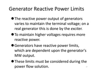
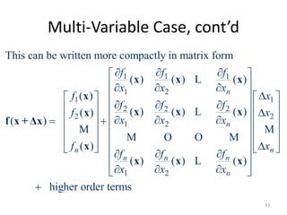
16. Two Bus PV Example, cont'd
( ) ( )* ( )
22 2
1
( ) ( )* ( ) ( )*
21 221 2 2 2
( )* ( )*
( 1) ( ) ( )2 2
2 212 1( )* ( )*
22 221, 22 2
(0)
2
( ) ( 1) ( 1)
2 2 2
Im ,
Im[ ]
1 1
Guess 1.05 0
0 0 0.457
k
n
v v
k
k
n
k k
k k
v v v
Q V Y V
Y V V Y V V
S S
V Y V Y V
Y YV V
V
v S V V
j

   
 
  
 


 
 
 
   
 
  
   
      
  
  


%
%
1.045 0.83 1.050 0.83
1 0 0.535 1.049 0.93 1.050 0.93
2 0 0.545 1.050 0.96 1.050 0.96
j
j
     
      
       16

17. Generator Reactive Power Limits
The reactive power output of generators
varies to maintain the terminal voltage; on a
real generator this is done by the exciter.
To maintain higher voltages requires more
reactive power.
Generators have reactive power limits,
which are dependent upon the generator's
MW output.
These limits must be considered during the
power flow solution. 17

18. Generator Reactive Limits, cont'd
During power flow once a solution is
obtained, need to check if the generator
reactive power output is within its limits
If the reactive power is outside of the limits,
then fix Q at the max or min value, and re-
solve treating the generator as a PQ bus
– this is know as "type-switching"
– also need to check if a PQ generator can again
regulate
Rule of thumb: to raise system voltage we
need to supply more VArs. 18

19. Accelerated G-S Convergence
( 1) ( )
( 1) ( ) ( ) ( )
(
Previously in the Gauss-Seidel method we were
calculating each value as
( )
To accelerate convergence we can rewrite this as
( )
Now introduce "acceleration parameter"
v v
v v v v
x
x h x
x x h x x
x




  
1) ( ) ( ) ( )
( ( ) )
With = 1 this is identical to standard Gauss-Seidel.
Larger values of may result in faster convergence.
v v v v
x h x x



  
19

20. Accelerated Convergence, cont’d
( 1) ( ) ( ) ( )
Consider the previous example: 1 0
(1 )
Matlab code: alpha=1.2;x=x0;x=x+alpha*(1+sqrt(x)-x).
Comparison of results with different values of
1 1.2 1.5 2
0 1 1 1 1
1 2 2.20 2.5 3
2
v v v v
x x
x x x x

    

  
   
   
2.4142 2.5399 2.6217 2.464
3 2.5554 2.6045 2.6179 2.675
4 2.5981 2.6157 2.6180 2.596
5 2.6118 2.6176 2.6180 2.626 20

21. Gauss-Seidel Advantages
Each iteration is relatively fast (computational
order is proportional to number of branches +
number of buses in the system).
Relatively easy to program.
21

22. Gauss-Seidel Disadvantages
Tends to converge relatively slowly, although
this can be improved with acceleration.
Has tendency to fail to find solutions,
particularly on large systems.
Tends to diverge on cases with negative
branch reactances (common with
compensated lines).
Need to program using complex numbers.
Gauss and Gauss-Seidel mostly replaced by
Newton-Raphson. 22

23. Newton-Raphson Algorithm
The second major power flow solution
method is the Newton-Raphson algorithm
Key idea behind Newton-Raphson is to use
sequential linearization
General form of problem: Find an such that
( ) 0
x
f x 
23

24. Newton-Raphson Method (scalar)
 
( )
( )
( ) ( ) ( ) ( ) ( )
2 2( ) ( )
2
1. Represent by a Taylor series about the
current guess . Write for the deviation
from :
( ) ( ) ( )
1
( )
2
higher order terms.
v v v v v
v v
f
x x
x
df
f x x f x x x
dx
d f
x x
dx



      
  
 
   
 
24

25. Newton-Raphson Method, cont’d
( ) ( ) ( ) ( ) ( )
( )
1
( ) ( ) ( )
2. Approximate by neglecting all terms
except the first two
( ) ( ) ( )
3. Set linear approximation equal to zero
and solve for
( ) ( )
4. Sol
v v v
v
v v v
f
df
f x x f x x x
dx
x
df
x x f x
dx
 

     
  

   
  
( 1) ( ) ( )
ve for a new estimate of solution:
v v v
x x x
   25

26. Newton-Raphson Example
2
1
( ) ( ) ( )
( ) ( ) 2
( )
( 1) ( ) ( )
( 1) ( ) ( ) 2
( )
Use Newton-Raphson to solve ( ) 0,
where: ( )= 2.
The iterative update is:
( ) ( )
1
(( ) 2)
2
1
(( ) 2).
2
v v v
v v
v
v v v
v v v
v
f x
f x x
df
x x f x
dx
x x
x
x x x
x x x
x





   
  
    
  
  
   
   26

27. Newton-Raphson Example, cont’d
( 1) ( ) ( ) 2
( )
(0)
( ) ( ) ( )
3 3
6
1
(( ) 2)
2
Matlab code: x=x0; x = x-(1/(2*x))*(x^2-2).
Guess 1. Iteratiting, we get:
( )
0 1 1 0.5
1 1.5 0.25 0.08333
2 1.41667 6.953 10 2.454 10
3 1.41422 6.024 10
v v v
v
v v v
x x x
x
x
x f x x

 

   
  




  

27

28. Sequential Linear Approximations
Function is f(x) = x2 - 2.
Solutions to f(x) = 0 are points where
f(x) intersects x axis.
At each
iteration the
N-R method
uses a linear
approximation
to determine
the next value
for x
28

29. Newton-Raphson Comments
• When close to the solution the error
decreases quite quickly -- method has what is
known as “quadratic” convergence:
– number of correct significant figures roughly
doubles at each iteration.
• f(x(v)) is known as the “mismatch,” which we
would like to drive to zero.
• Stopping criteria is when f(x(v))  < 
29

30. Newton-Raphson Comments
• Results are dependent upon the initial guess.
What if we had guessed x(0) = 0, or x(0) = -1?
• A solution’s region of attraction (ROA) is the
set of initial guesses that converge to the
particular solution.
• The ROA is often hard to determine.
30

31. Multi-Variable Newton-Raphson
1 1
2 2
Next we generalize to the case where is an -
dimension vector, and ( ) is an -dimensional
vector function:
( )
( )
( )
( )
Again we seek a solution of ( ) 0.
n n
n
n
x f
x f
x f
   
   
    
   
   
   

x
f x
x
x
x f x
x
f x
M M
31

32. Multi-Variable Case, cont’d
i
1 1
1 1 1 2
1 2
1
1 2
1 2
The Taylor series expansion is written for each f ( )
( ) ( ) ( ) ( )
( ) higher order terms
( ) ( ) ( ) ( )
( ) higher order terms
n
n
n n
n n
n
n
n
f f
f x x f x x x x x
x x
f
x x
x
f f
f x x f x x x x x
x x
f
x x
x
 
       
 

 

 
       
 

 

x
M
32

33. Multi-Variable Case, cont’d
1 1 1
1 2
1 1
2 2 2
2 2
1 2
1 2
This can be written more compactly in matrix form
( ) ( ) ( )
( )
( ) ( ) ( )( )
( )
( )
( ) ( ) ( )
n
n
n
n n n
n
f f f
x x x
f x
f f f
f x
x x x
f
f f f
x x x
   
   
  
     
      
  
  
     
 
   
x x x
x
x x xx
f x + Δx
x
x x x
L
L
M
M O O M
L
higher order terms
nx
 
 
 
 
  

M
33

34. Jacobian Matrix
1 1 1
1 2
2 2 2
1 2
1 2
The by matrix of partial derivatives is known
as the Jacobian matrix, ( )
( ) ( ) ( )
( ) ( ) ( )
( )
( ) ( ) ( )
n
n
n n n
n
n n
f f f
x x x
f f f
x x x
f f f
x x x
   
   
 
   
   
 
 
   
 
    
J x
x x x
x x x
J x
x x x
L
L
M O O M
L
34

35. Multi-Variable N-R Procedure
Derivation of N-R method is similar to the scalar case
( ) ( ) ( ) higher order terms
( ) ( ) ( )
To seek solution to ( ) 0, set linear
approximation equal to zero: 0 ( ) ( ) .
     
    
  
  
  
f x x f x J x x
f x x f x J x x
f x x
f x J x x
x 1
( 1) ( ) ( )
( 1) ( ) ( ) 1 ( )
( )
( ) ( )
( ) ( )
Iterate until ( )
v v v
v v v v
v



 
  
 

J x f x
x x x
x x J x f x
f x
35

36. Multi-Variable Example
1
2
2 2
1 1 2
2 2
2 1 2 1 2
1 1
1 2
2 2
1 2
Solve for = such that ( ) 0 where
( ) 2 8
( ) 4
First symbolically determine the Jacobian
( ) ( )
( ) =
( ) ( )
x
x
f x x x
f x x x x x
f f
x x
x x
f f
x x
x x
 
 
 
  
   
  
  
 
  
   
x f x
J x
36

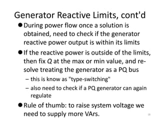
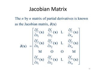
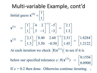
37. Multi-variable Example, cont’d
1 2
1 2 1 2
1
1 1 2 1
2 1 2 1 2 2
4 2
( ) =
2 2
4 2 ( )
Then
2 2 ( )
Matlab code: x1=x10; x2=x20;
f1=2*x1^2+x2^2-8;
f2=x1^2-x2^2+x1*x2-4;
J = [4*x1 2*x2; 2*x1+x2 x1-2*x2];
[x1;x2] =
x x
x x x x
x x x f
x x x x x f

 
   
     
             
J x
x
x
[x1;x2]-inv(J)*[f1;f2].
37

38. Multi-variable Example, cont’d
(0)
1
(1)
1
(2)
( )
1
Initial guess
1
1 4 2 5 2.1
1 3 1 3 1.3
2.1 8.40 2.60 2.51 1.8284
1.3 5.50 0.50 1.45 1.2122
At each iteration we check ( ) to see if it


 
  
 
       
                 
       
                
x
x
x
f x
(2)
is
0.1556
below our specified tolerance : ( )
0.0900
If = 0.2 then done. Otherwise continue iterating.


 
  
 
f x
38