2d beam element with combined loading bending axial and torsion
The document discusses beam theory and finite element modeling of beams and frames. It provides information on modeling beams using one-dimensional beam elements with cubic shape functions. The formulation describes defining the element stiffness matrix and calculating the element's contribution to the global structural stiffness matrix and force vector based on applied loads. Boundary conditions and sample problems are presented to demonstrate the element modeling approach.
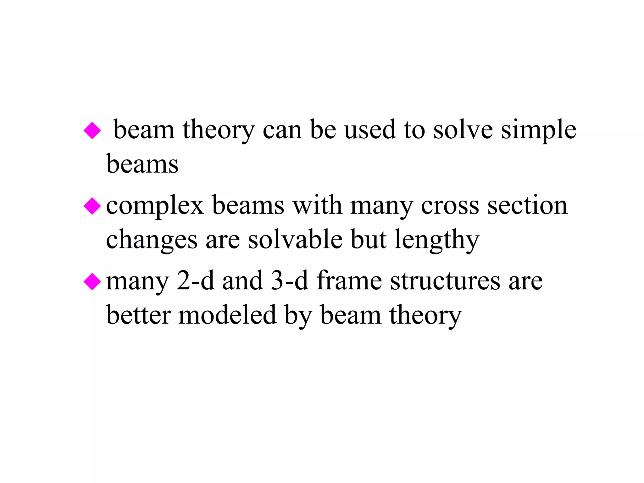
beam theorycan be used to solve simple
beams
complex beams with many cross section
changes are solvable but lengthy
many 2-d and 3-d frame structures are
better modeled by beam theory
3.
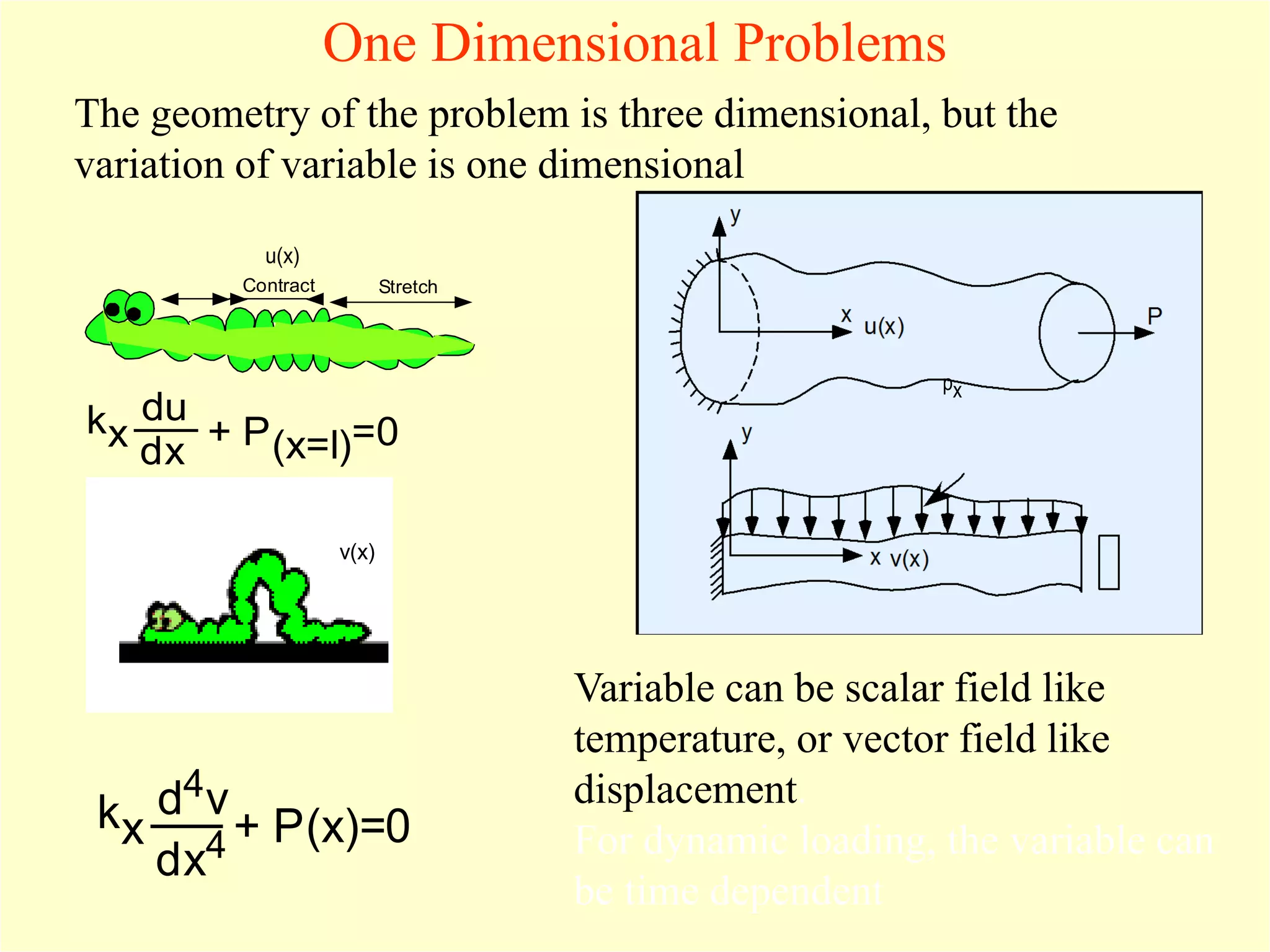
One Dimensional Problems
px
StretchContract
u(x)
v(x)
kx+ P(x=l)=0
du
dx
kx + P(x)=0
d4v
dx4
Variable can be scalar field like
temperature, or vector field like
displacement.
For dynamic loading, the variable can
be time dependent
The geometry of the problem is three dimensional, but the
variation of variable is one dimensional
4.
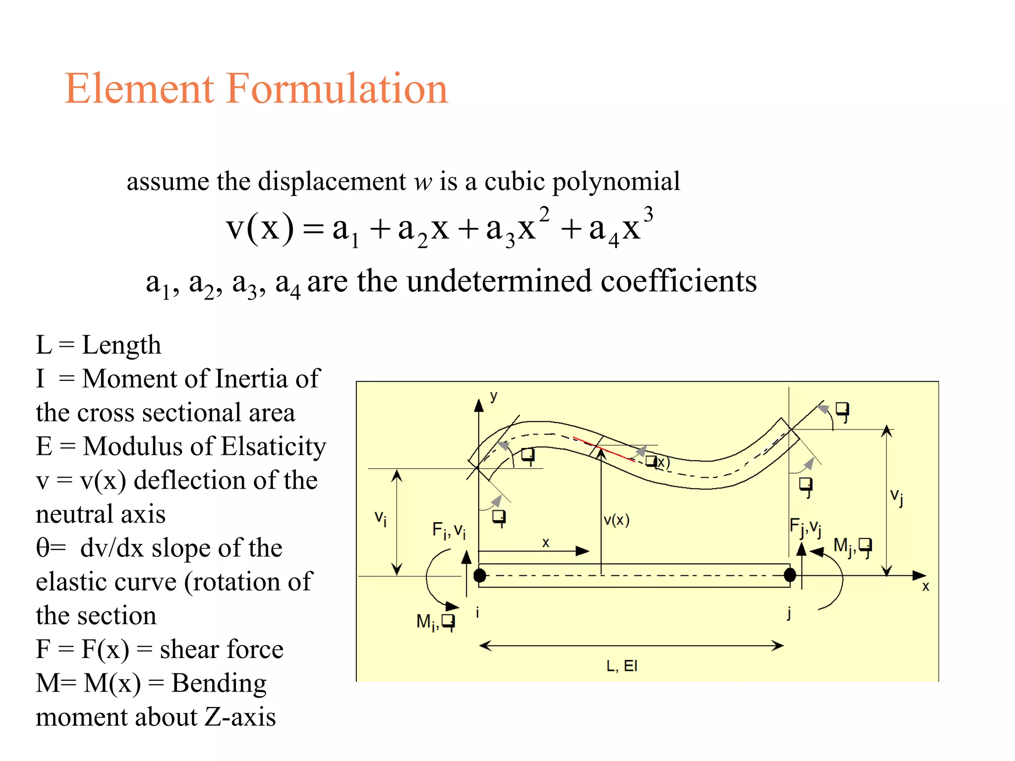
Element Formulation
– assumethe displacement w is a cubic polynomial in
L = Length
I = Moment of Inertia of
the cross sectional area
E = Modulus of Elsaticity
v = v(x) deflection of the
neutral axis
θ= dv/dx slope of the
elastic curve (rotation of
the section
F = F(x) = shear force
M= M(x) = Bending
moment about Z-axis
a1, a2, a3, a4 are the undetermined coefficients
2 3
1 2 3 4v(x) a a x a x a x= + + +
5.
`
1 1
x 0
22
x L
dv
x 0, v(0) v ;
dx
dv
x L, v(L) v ;
dx
=
=
= = = θ
= = = θ
{ } { }
1 1
2 22 3 2
3 3
4 4
a a
a a
v(x) 1 x x x ; (x) 0 1 2x 3x
a a
a a
θ=
i 1
i 2
2 3
j 3
2
j 4
v 1 0 0 0 a
0 1 0 0 a
v a1 L L L
a0 1 2L 3L
θ
=
θ
6.
Applying theseboundary conditions, we get
Substituting coefficients ai back into the original equation
for v(x) and rearranging terms gives
1
1 1 2 1
3 1 1 2 22
{d} [P(x)]{a}
{a} [P(x)] {d}
a v ; a
1
a ( 3v 2L 3v L )
L
−
=
=
= = θ
= − − θ + − θ
{ }
1
22 3
3
4
a
a
v(x) 1 x x x
a
a
=
7.
The interpolationfunction or shape function is given by
2 3 2 3
1 12 3 2
2 3 2 3
2 22 3 2
3x 2x 2x x
v(x) (1 )v (x )
L L L L
3x 2x x x
( )v ( )
L L L L
= − + + − + θ
+ − + − + θ
[ ]
1
1
1 2 3 4
2
2
v
L
v N (x) N (x) N (x) N (x) [N]{d}
v
L
θ
=
θ
8.
strain for abeam in bending is defined by the curvature, so
Hence
2 2
2 2
du d v d [N]
y {d} y[B]{d}
dx dx dx
ε= = = =
{ } { }
{ } [ ]{ }
{ } [ ]{ }
{ } [ ] { }
{ } [ ] [ ][ ]{ }
e
e
e
T
e
v
Te
v
T Te 2
v
Internal virtual energy U = dv
substitute E in above eqn.
U = E dv
= y B d
U = d B E B d y dv
δ δ ε σ
σ= ε
δ δ ε ε
δ ε δ
δ δ
∫
∫
∫
3 2 3 2 2 3 3 2
12x 6 6x 4 6 12x 6x 2
[B]
L L L L L L L h
= − − − −
9.
{ } [] [ ][ ] { } { } [ ] { } [ ] { } { }
{ } { }
[ ] [ ][ ]
{ } [ ] { } [ ] { } { }
e eFrom virtual work principle U W
T TT T T2 ed ( B E B y dv d d N b dv N p dv P
y y
e e sv v
eK U F
e e
where
T 2K B D B y dv Element stiffness matrix
e
ev
T T eF N b dv N p ds P Total nodal force vector
e y y
e sv
δ =δ
δ =δ + +∫ ∫ ∫
⇒ =
=∫
+ +=∫ ∫
{ } { } { } [ ] { }
{ } { } { } [ ] { }
{ } { } { }
e e
T T Te
b y
v v
T T Te
s y
s s
TTe e e
c
External virtual workdue to body force
w = d(x) b dv d N b dv
External virtual work due to surface force
w = d(x) p dv d N p ds
External virtual work due to nodal forces
w d P , P
δ δ =δ
δ δ =δ
δ =δ
∫ ∫
∫ ∫
{ }yi i yj= P , M ,P ,....
10.
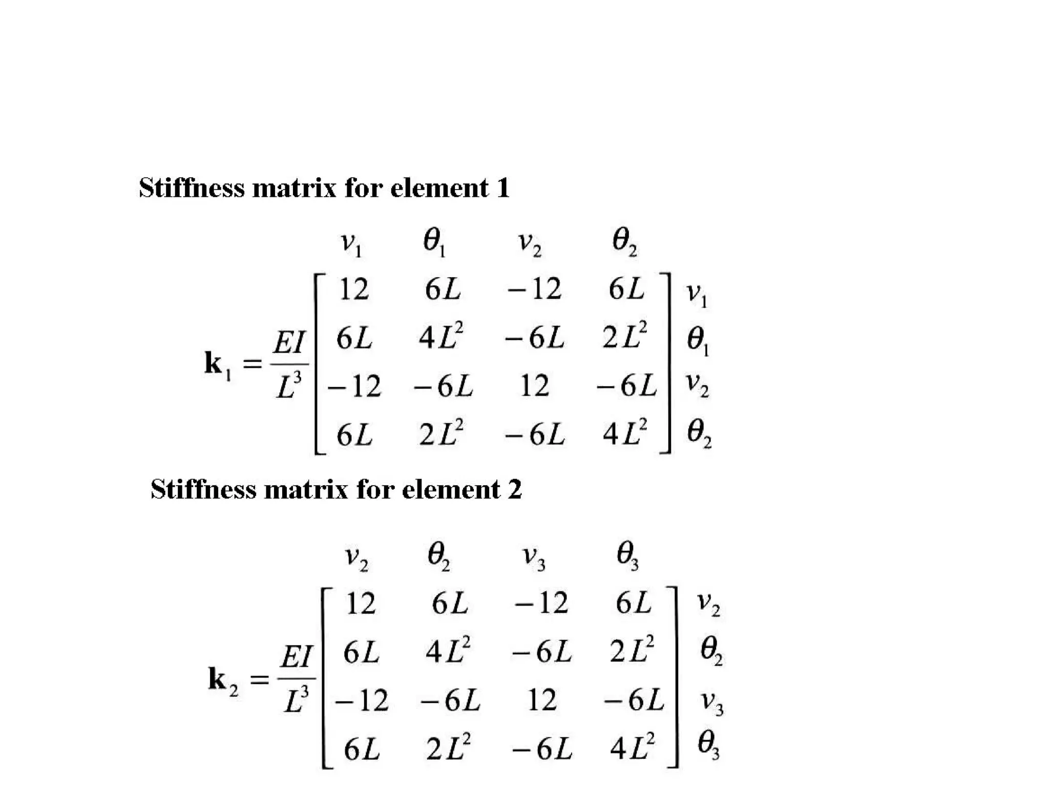
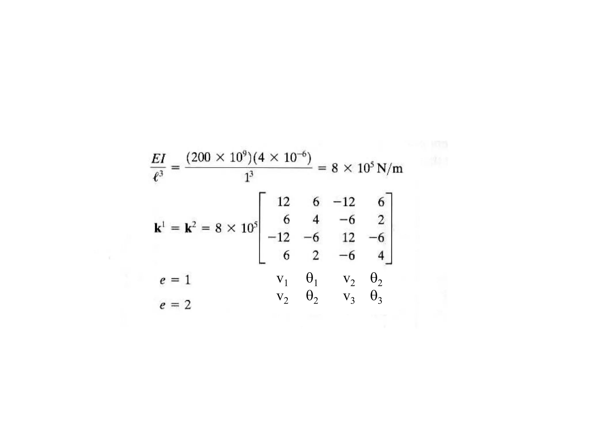
the stiffness matrix[k] is defined
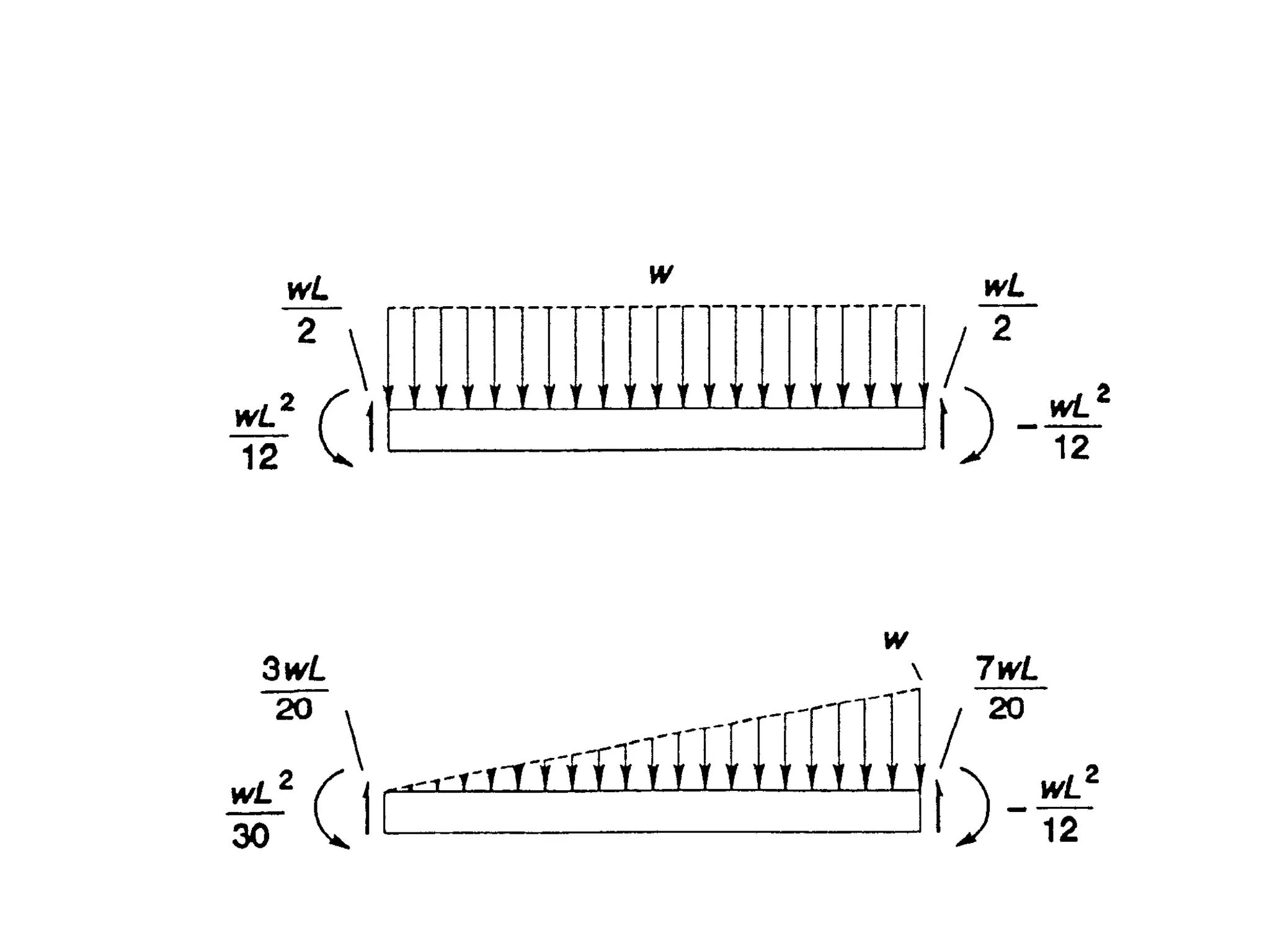
To compute equivalent nodal force vector
for the loading shown
{ } [ ] { }
[ ]
T
e y
s
y
y
2 3 2 3 2 3 2 3
2 3 2 2 3 2
F N p ds
From similar triangles
p w w
; p x; ds = 1 dx
x L L
3x 2x 2x x 3x 2x x x
N (1 ) (x ) ( ) ( )
L L L L L L L L
=
= = ⋅
= − + − + − − +
∫
w
x
py
L
( )
L
T 2 T
V
A 0
2 2
3
2 2
[k] [B] E[B]dV dAy E [B] [B]dx
12 6L 12 6L
6L 4L 6L 2LEI
12 6L 12 6LL
6L 2L 6L 4L
= =
−
−
=
− − −
−
∫ ∫ ∫
11.
{ } [] { }
{ }
T
e y
s
2 3
2 3
22 3
2
e 2 3
L
2 3
22 3
2
F N p ds
3wL3x 2x
(1 )
20L L
wL2x x
(x )
wx 30L L
F dx
7wLL3x 2x
( )
20L L
wLx x
( )
20L L
=
−− +
−− +
−=
−−
− +
∫
∫
+ve directions
vi vj
qi qj
w
Equivalent nodal force due to
Uniformly distributed load w
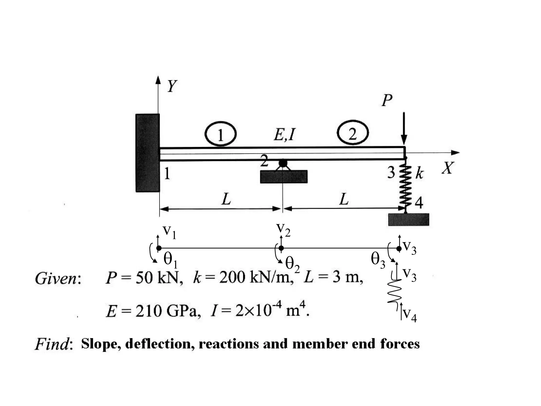
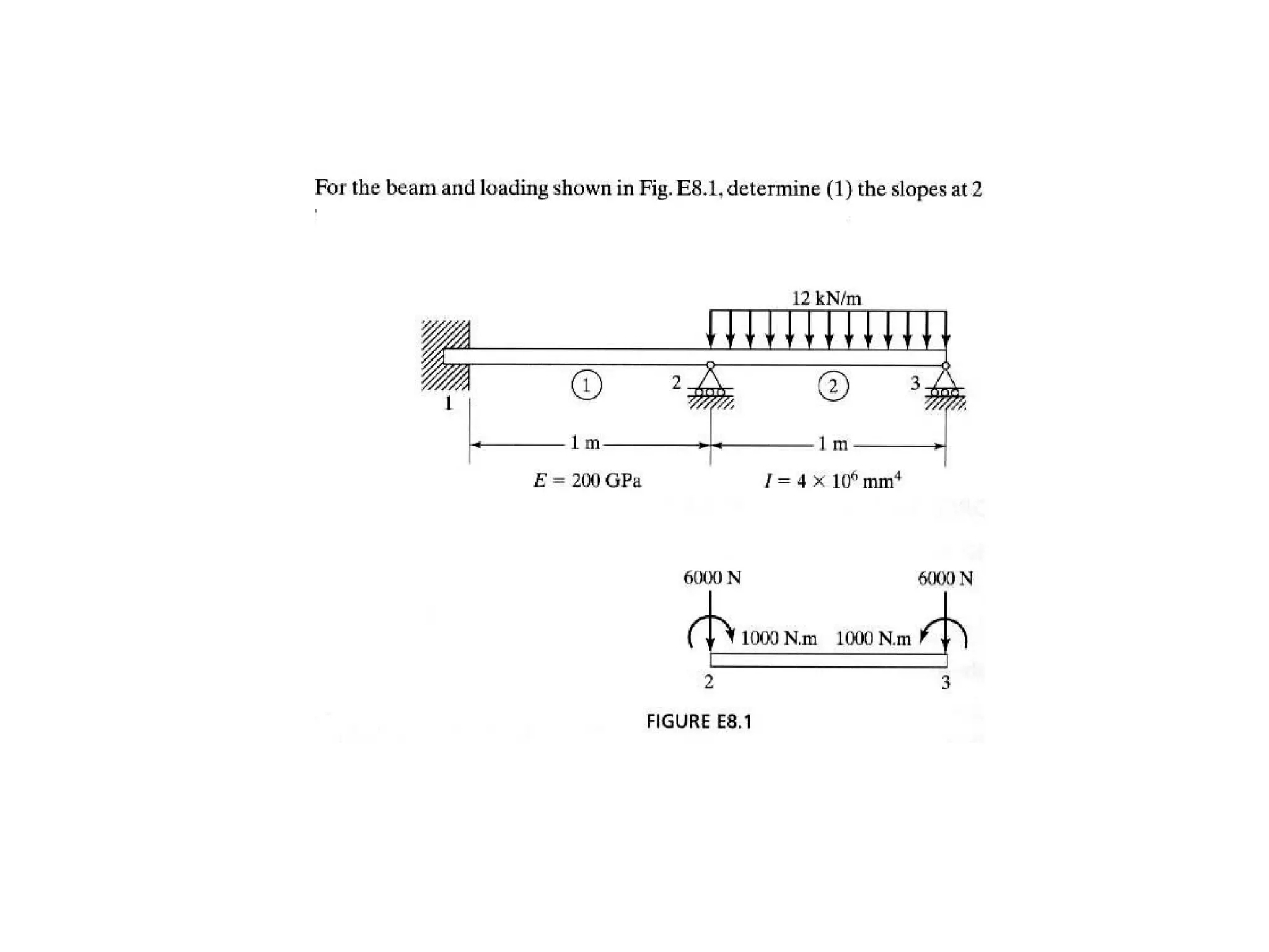
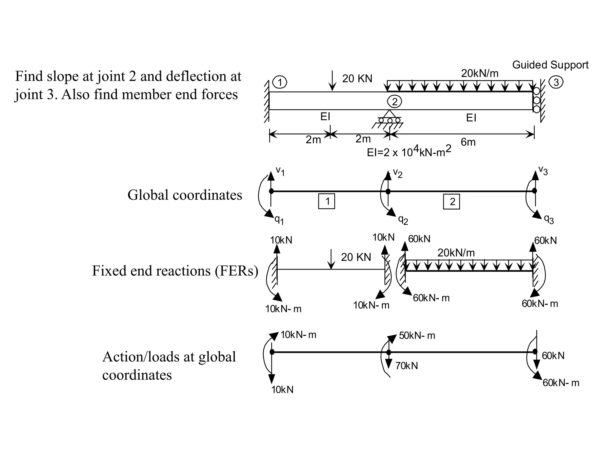
Find slope atjoint 2 and deflection at
joint 3. Also find member end forces
1
1
20 KN 20kN/m
10kN 10kN
10kN- m 10kN- m
60kN- m
60kN- m
60kN 60kN
v1
q1 q2 q3
v2
v3
EI EI
20 KN 20kN/m
Guided Support
2m 2m 6m
EI=2 x 10⁴kN-m2
10kN- m
10kN
70kN
50kN- m
60kN- m
60kN
2
2
3
Global coordinates
Fixed end reactions (FERs)
Action/loads at global
coordinates
{ } []{ }
If f ' member end forces in local coordinates then
f' k' q'=
3 3 3 3
3 3 3 3
3 3 3 3
3 3 3 3
AE AE
0 0 0 0
L L
12EI 6EI 12EI 6EI
0 0
L L L L
6EI 4EI 6EI 2EI
0 0
L L L L[k]
AE AE
0 0 0 0
L L
12EI 6EI 12EI 6EI
0 0
L L L L
6EI 2EI 6EI 4EI
0 0
L L L L
−
−
−
=
−
− − −
−
30.
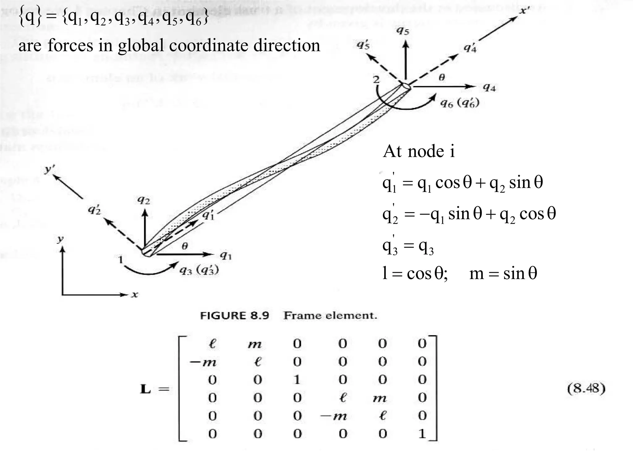
'
1 1 2
'
21 2
'
3 3
At node i
q q cos q sin
q q sin q cos
q q
l cos ; m sin
= θ + θ
= − θ + θ
=
= θ = θ
{ } 1 2 3 4 5 6q {q ,q ,q ,q ,q ,q }
are forces in global coordinate direction
=
31.
{ } {}
[ ] [ ] [ ][ ]T
using conditions q' [L]{q}; and f' [L]{f}
Stiffness matrix for an arbitrarily oriented beam element is given by
k L k' L
= =
=
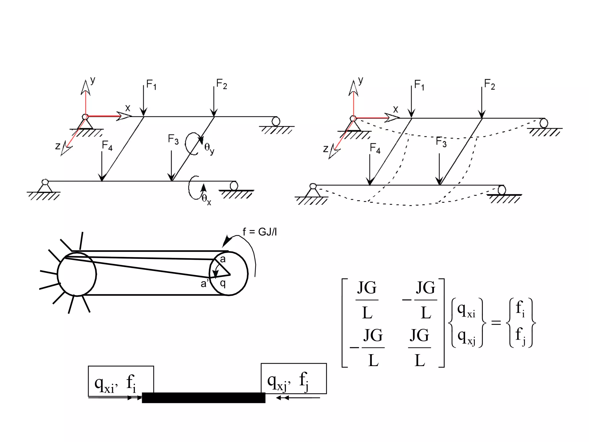
32.
a
a’ q
f =GJ/l
qxi’ fi
qxj’ fj
Grid Elements
xi i
xj j
JG JG
q fL L
q fJG JG
L L
−
=
−
34.
{ } []{ }
If f ' member end forces in local coordinates then
f' k' q'=
3 3 3 3
3 3 3 3
3 3 3 3
3 3 3 3
GJ GJ
0 0 0 0
L L
12EI 6EI 12EI 6EI
0 0
L L L L
6EI 4EI 6EI 2EI
0 0
L L L L
GJ GJ
0 0 0 0
L L
12EI 6EI 12EI 6EI
0 0
L L L L
6EI 2EI 6EI 4EI
0 0
L L L L
−
−
−
−
− − −
−
35.
[ ]
C 0-s 0 0 0
0 1 0 0 0 0
-s 0 c 0 0 0
L
0 0 0 c 0 -s
0 0 0 0 1 0
0 0 0 --s 0 c
=
[ ] [ ] [ ][ ]T
k L k' L
=
if axial loadis tensile, results from beam
elements are higher than actual ⇒ results
are conservative
if axial load is compressive, results are less
than actual
– size of error is small until load is about 25% of
Euler buckling load
41.
for 2-d, canuse rotation matrices to get
stiffness matrix for beams in any
orientation
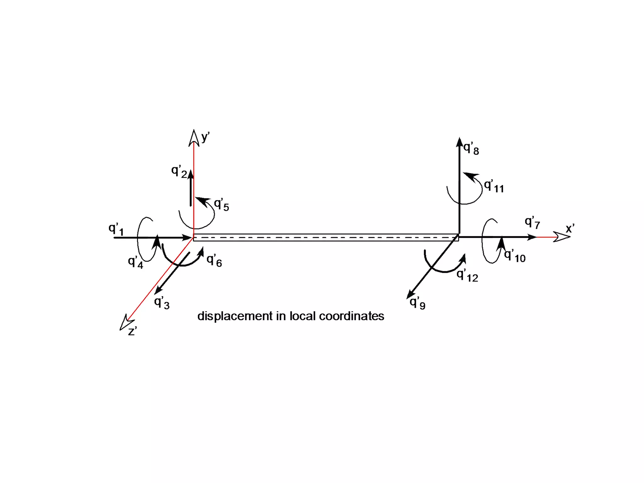
to develop 3-d beam elements, must also
add capability for torsional loads about the
axis of the element, and flexural loading in
x-z plane
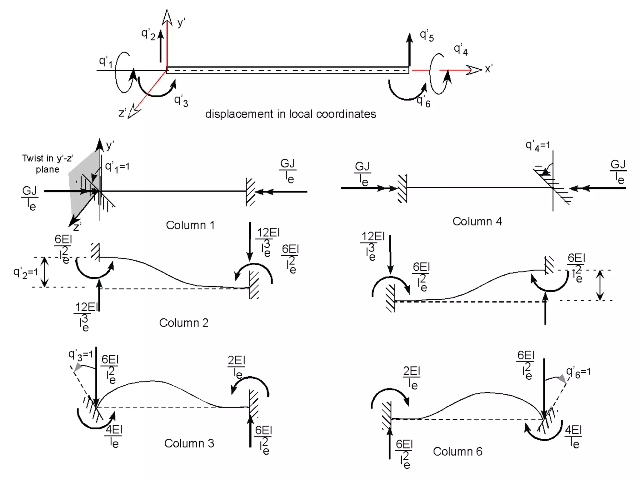
42.
to derive the3-d beam element, set up the
beam with the x axis along its length, and y
and z axes as lateral directions
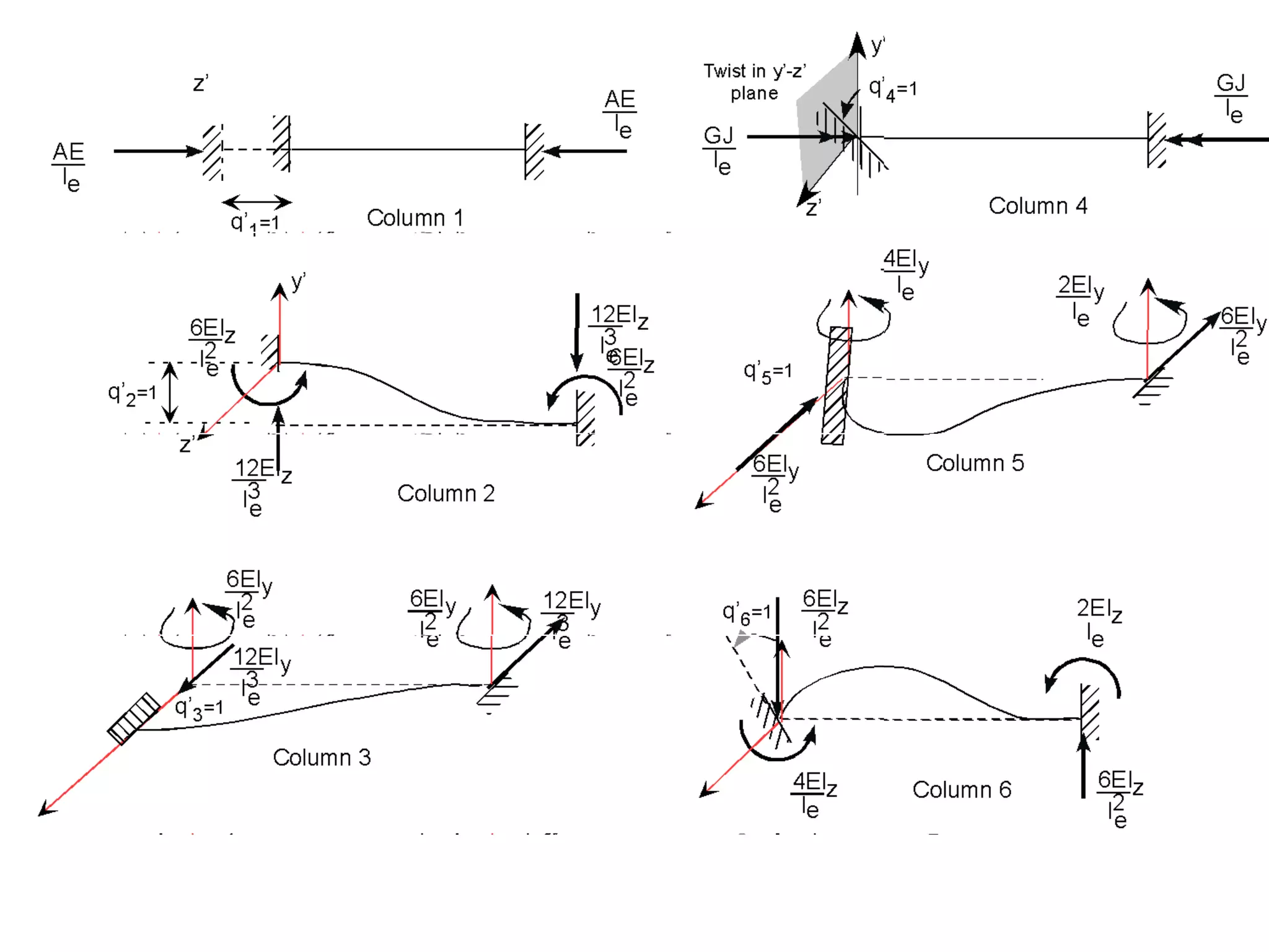
torsion behavior is added by superposition
of simple strength of materials solution
JG
L
JG
L
JG
L
JG
L
T
T
xi
xj
i
j
−
−
=
φ
φ
43.
J = torsionalmoment about x axis
G = shear modulus
L = length
φxi, φxj are nodal degrees of freedom of
angle of twist at each end
Ti, Tj are torques about the x axis at each
end
44.
flexure in x-zplane adds another stiffness
matrix like the first one derived
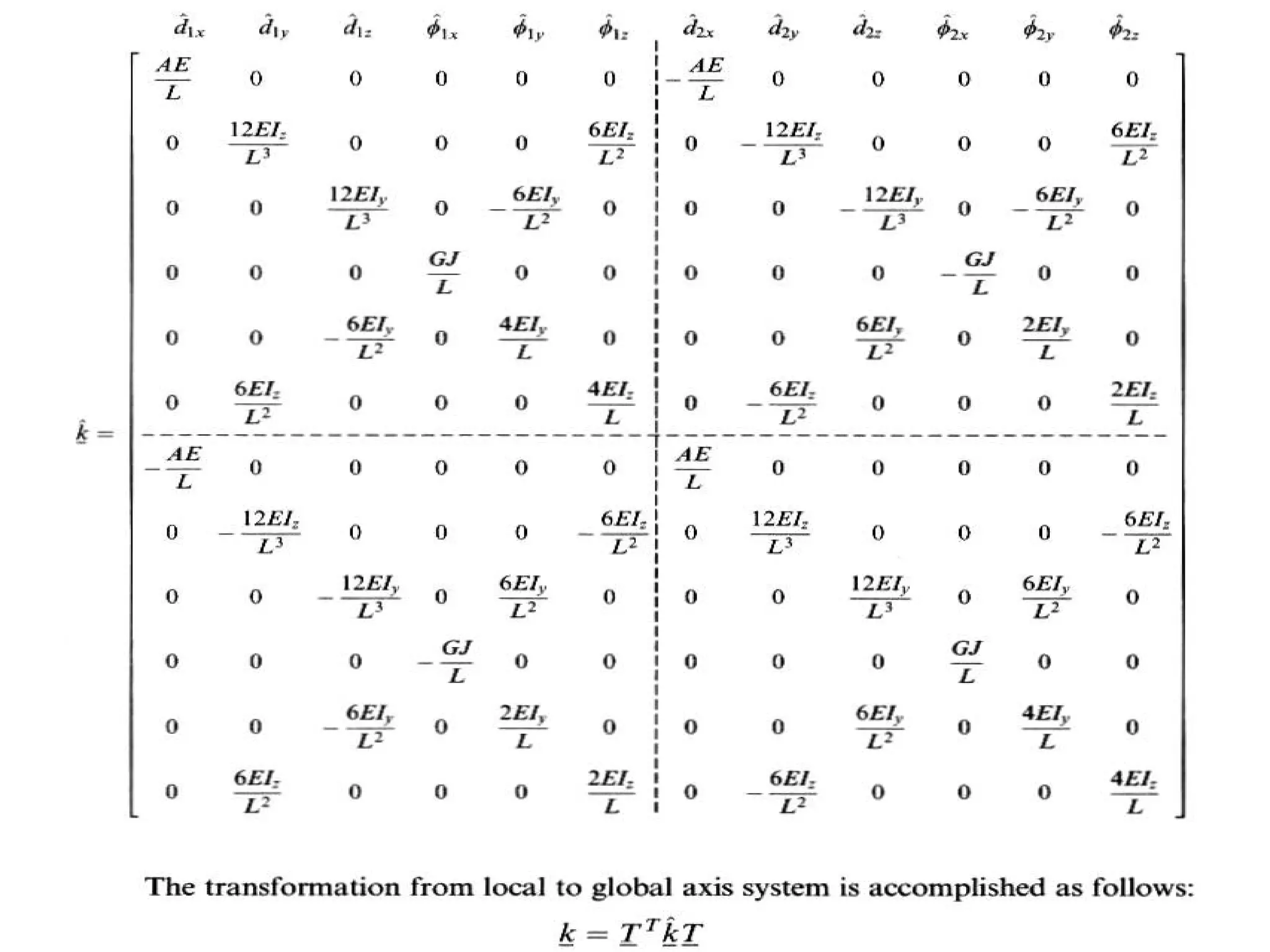
superposition of all these matrices gives a
12 × 12 stiffness matrix
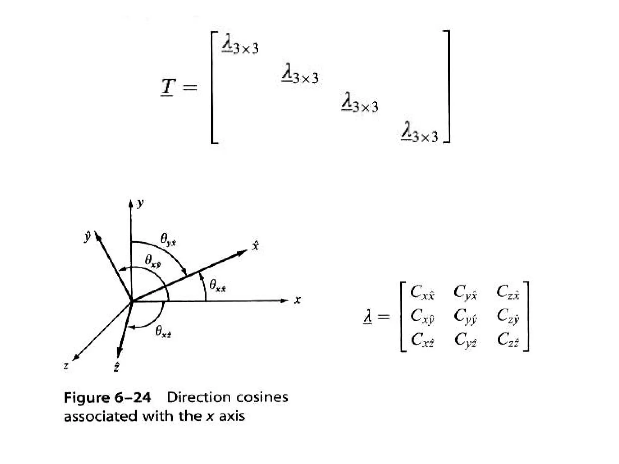
to orient a beam element in 3-d, use 3-d
rotation matrices
45.
for beams longcompared to their cross
section, displacement is almost all due to
flexure of beam
for short beams there is an additional lateral
displacement due to transverse shear
some FE programs take this into account,
but you then need to input a shear
deformation constant (value associated with
geometry of cross section)
46.
limitations:
– same assumptionsas in conventional beam and
torsion theories
⇒no better than beam analysis
– axial load capability allows frame analysis, but
formulation does not couple axial and lateral
loading which are coupled nonlinearly
47.
– analysis doesnot account for
» stress concentration at cross section changes
» where point loads are applied
» where the beam frame components are connected
48.
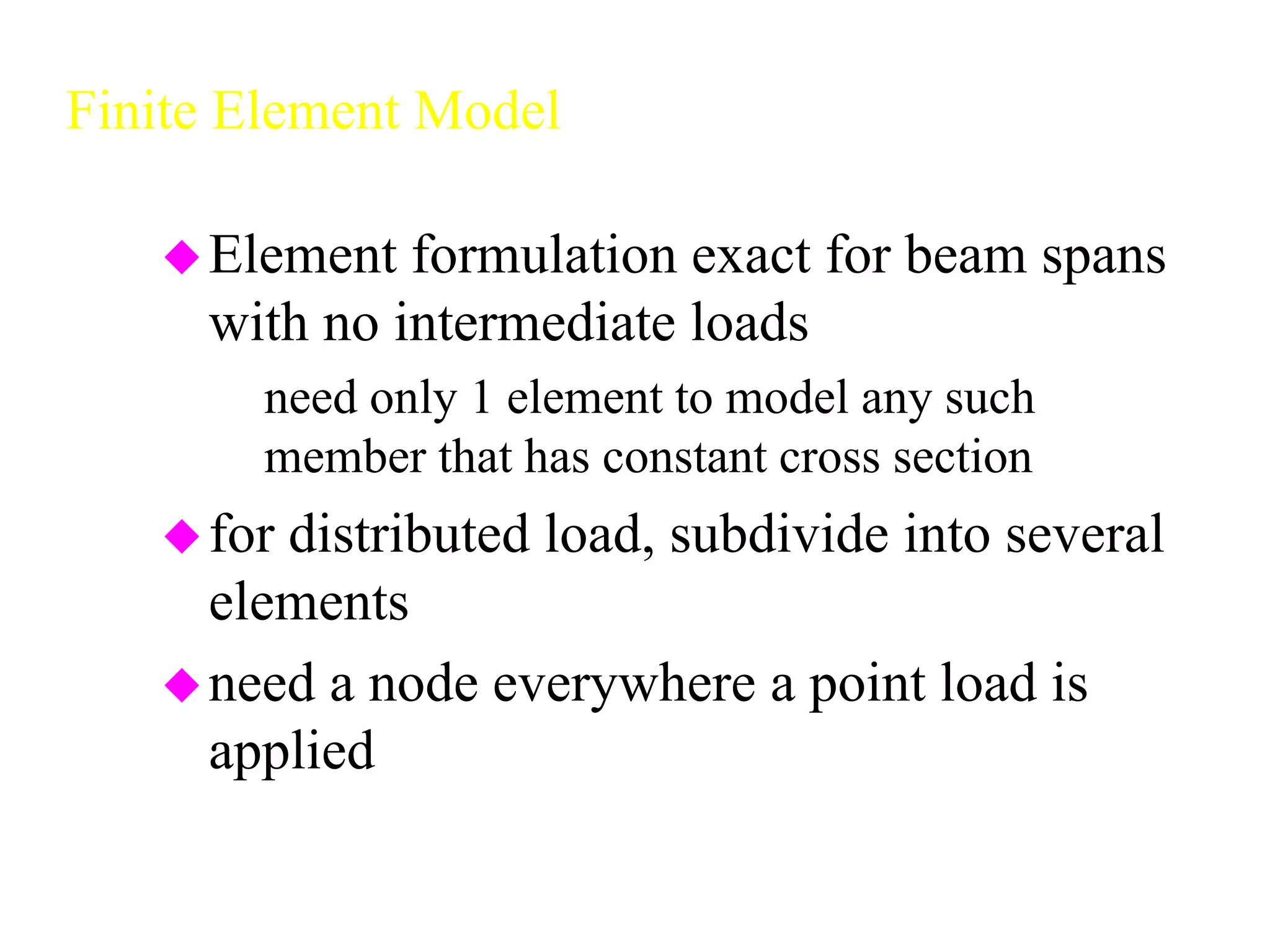
Finite Element Model
Elementformulation exact for beam spans
with no intermediate loads
– need only 1 element to model any such
member that has constant cross section
for distributed load, subdivide into several
elements
need a node everywhere a point load is
applied
49.
need nodes whereframe members connect,
where they change direction, or where the
cross section properties change
for each member at a common node, all
have the same linear and rotational
displacement
boundary conditions can be restraints on
linear displacements or rotation
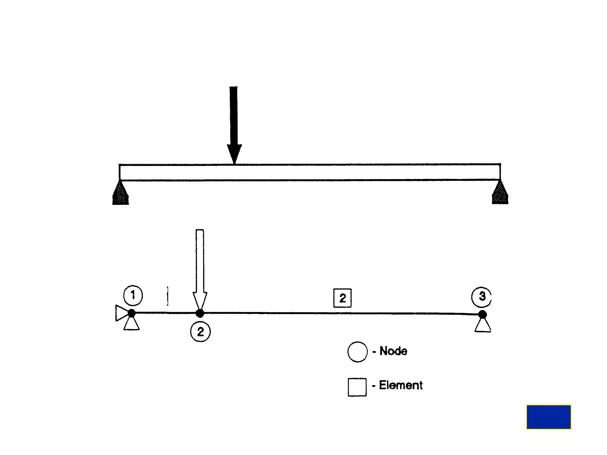
– restrain verticaland horizontal displacements
of nodes 1 and 3
– no restraint on rotation of nodes 1 and 3
– need a restraint in x direction to prevent rigid
body motion, even if all forces are in y
direction
53.
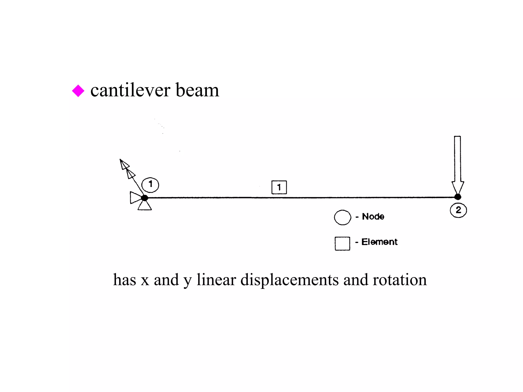
cantilever beam
–has x and y linear displacements and rotation of node 1
fixed
54.
point loads areidealized loads
– structure away from area of application
behaves as though point loads are applied
55.
only an exactformulation when there are no
loads along the span
– for distributed loads, can get exact solution
everywhere else by replacing the distributed
load by equivalent loads and moments at the
nodes
57.
Computer Input Assistance
preprocessorwill usually have the same
capabilities as for trusses
a beam element consists of two node
numbers and associated material and
physical properties
58.
material properties:
– modulusof elasticity
– if dynamic or thermal analysis, mass density
and thermal coefficient of expansion
physical properties:
– cross sectional area
– 2 area moments of inertia
– torsion constant
– location of stress calculation point
59.
boundary conditions:
– specifynode numbers and displacement
components that are restrained
loads:
– specify by node number and load components
– most commercial FE programs allows
application of distributed loads but they use
and equivalent load/moment set internally
60.
Analysis Step
small modelsand carefully planned element
and node numbering will save you from
bandwidth or wavefront minimization
potential for ill conditioned stiffness matrix
due to axial stiffness >> flexural stiffness
(case of long slender beams)
61.
Output Processing andEvaluation
graphical output of deformed shape usually
uses only straight lines to represent
members
you do not see the effect of rotational
constraints on the deformed shape of each
member
to check these, subdivide each member and
redo the analysis
62.
most FEcodes do not make graphical
presentations of beam stress results
– user must calculate some of these from the stress
values returned
for 2-d beams, you get a normal stress normal to
the cross section and a transverse shear acting on
the face of the cross section
– normal stress has 2 components
» axial stress
» bending stress due to moment
63.
– expect themaximum normal stress to be at the
top or bottom of the cross section
– transverse shear is usually the average
transverse load/area
» does not take into account any variation across the
section
64.
3-d beams
– normalstress is combination of axial stress,
flexural stress from local y- and z- moments
– stress due to moment is linear across a section,
the combination is usually highest at the
extreme corners of the cross section
– may also have to include the effects of torsion
» get a 2-d stress state which must be evaluated
– also need to check for column buckling
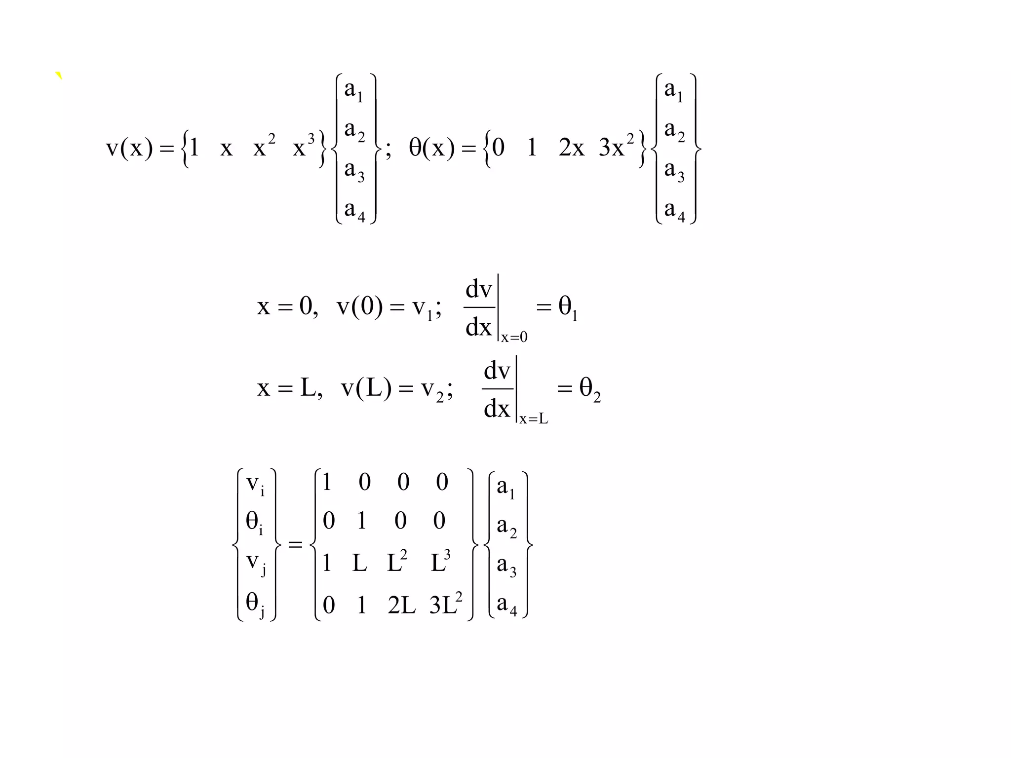
![ Applying these boundary conditions, we get
Substituting coefficients ai back into the original equation
for v(x) and rearranging terms gives
1
1 1 2 1
3 1 1 2 22
{d} [P(x)]{a}
{a} [P(x)] {d}
a v ; a
1
a ( 3v 2L 3v L )
L
−
=
=
= = θ
= − − θ + − θ
{ }
1
22 3
3
4
a
a
v(x) 1 x x x
a
a
=
](https://image.slidesharecdn.com/2dbeamelementwithcombinedloadingbendingaxialandtorsion-170720044252/75/2d-beam-element-with-combined-loading-bending-axial-and-torsion-6-2048.jpg)
![ The interpolation function or shape function is given by
2 3 2 3
1 12 3 2
2 3 2 3
2 22 3 2
3x 2x 2x x
v(x) (1 )v (x )
L L L L
3x 2x x x
( )v ( )
L L L L
= − + + − + θ
+ − + − + θ
[ ]
1
1
1 2 3 4
2
2
v
L
v N (x) N (x) N (x) N (x) [N]{d}
v
L
θ
=
θ ](https://image.slidesharecdn.com/2dbeamelementwithcombinedloadingbendingaxialandtorsion-170720044252/75/2d-beam-element-with-combined-loading-bending-axial-and-torsion-7-2048.jpg)
![strain for a beam in bending is defined by the curvature, so
Hence
2 2
2 2
du d v d [N]
y {d} y[B]{d}
dx dx dx
ε= = = =
{ } { }
{ } [ ]{ }
{ } [ ]{ }
{ } [ ] { }
{ } [ ] [ ][ ]{ }
e
e
e
T
e
v
Te
v
T Te 2
v
Internal virtual energy U = dv
substitute E in above eqn.
U = E dv
= y B d
U = d B E B d y dv
δ δ ε σ
σ= ε
δ δ ε ε
δ ε δ
δ δ
∫
∫
∫
3 2 3 2 2 3 3 2
12x 6 6x 4 6 12x 6x 2
[B]
L L L L L L L h
= − − − − ](https://image.slidesharecdn.com/2dbeamelementwithcombinedloadingbendingaxialandtorsion-170720044252/75/2d-beam-element-with-combined-loading-bending-axial-and-torsion-8-2048.jpg)
![{ } [ ] [ ][ ] { } { } [ ] { } [ ] { } { }
{ } { }
[ ] [ ][ ]
{ } [ ] { } [ ] { } { }
e eFrom virtual work principle U W
T TT T T2 ed ( B E B y dv d d N b dv N p dv P
y y
e e sv v
eK U F
e e
where
T 2K B D B y dv Element stiffness matrix
e
ev
T T eF N b dv N p ds P Total nodal force vector
e y y
e sv
δ =δ
δ =δ + +∫ ∫ ∫
⇒ =
=∫
+ +=∫ ∫
{ } { } { } [ ] { }
{ } { } { } [ ] { }
{ } { } { }
e e
T T Te
b y
v v
T T Te
s y
s s
TTe e e
c
External virtual workdue to body force
w = d(x) b dv d N b dv
External virtual work due to surface force
w = d(x) p dv d N p ds
External virtual work due to nodal forces
w d P , P
δ δ =δ
δ δ =δ
δ =δ
∫ ∫
∫ ∫
{ }yi i yj= P , M ,P ,....](https://image.slidesharecdn.com/2dbeamelementwithcombinedloadingbendingaxialandtorsion-170720044252/75/2d-beam-element-with-combined-loading-bending-axial-and-torsion-9-2048.jpg)
![the stiffness matrix [k] is defined
To compute equivalent nodal force vector
for the loading shown
{ } [ ] { }
[ ]
T
e y
s
y
y
2 3 2 3 2 3 2 3
2 3 2 2 3 2
F N p ds
From similar triangles
p w w
; p x; ds = 1 dx
x L L
3x 2x 2x x 3x 2x x x
N (1 ) (x ) ( ) ( )
L L L L L L L L
=
= = ⋅
= − + − + − − +
∫
w
x
py
L
( )
L
T 2 T
V
A 0
2 2
3
2 2
[k] [B] E[B]dV dAy E [B] [B]dx
12 6L 12 6L
6L 4L 6L 2LEI
12 6L 12 6LL
6L 2L 6L 4L
= =
−
−
=
− − −
−
∫ ∫ ∫](https://image.slidesharecdn.com/2dbeamelementwithcombinedloadingbendingaxialandtorsion-170720044252/75/2d-beam-element-with-combined-loading-bending-axial-and-torsion-10-2048.jpg)
![{ } [ ] { }
{ }
T
e y
s
2 3
2 3
22 3
2
e 2 3
L
2 3
22 3
2
F N p ds
3wL3x 2x
(1 )
20L L
wL2x x
(x )
wx 30L L
F dx
7wLL3x 2x
( )
20L L
wLx x
( )
20L L
=
−− +
−− +
−=
−−
− +
∫
∫
+ve directions
vi vj
qi qj
w
Equivalent nodal force due to
Uniformly distributed load w](https://image.slidesharecdn.com/2dbeamelementwithcombinedloadingbendingaxialandtorsion-170720044252/75/2d-beam-element-with-combined-loading-bending-axial-and-torsion-11-2048.jpg)
![1
1
2 5
2
3
3
V 12 6 -12 6
M 6 4 -6 2
V -12 -6 12+12 -6+6 -12 6
8x10
M 6 2 -6+6 4+4 -6 2
-12 -6V
M
=
1
1
2
2
3
3
1 1 2 3
2 3
5
v
v
12 -6 v
6 2 -6 4
Boundary condition
v , ,v ,v 0
Loading Condition
M 1000; M 1000
8 2
8x10
2
θ
θ
θ
θ =
=− =
{ } [ ]{ }
2
3
4
2
5 4
3
1000
4 1000.0
4 -2 1000 2.679x101
-2 8 1000.028*8x10 4.464x10
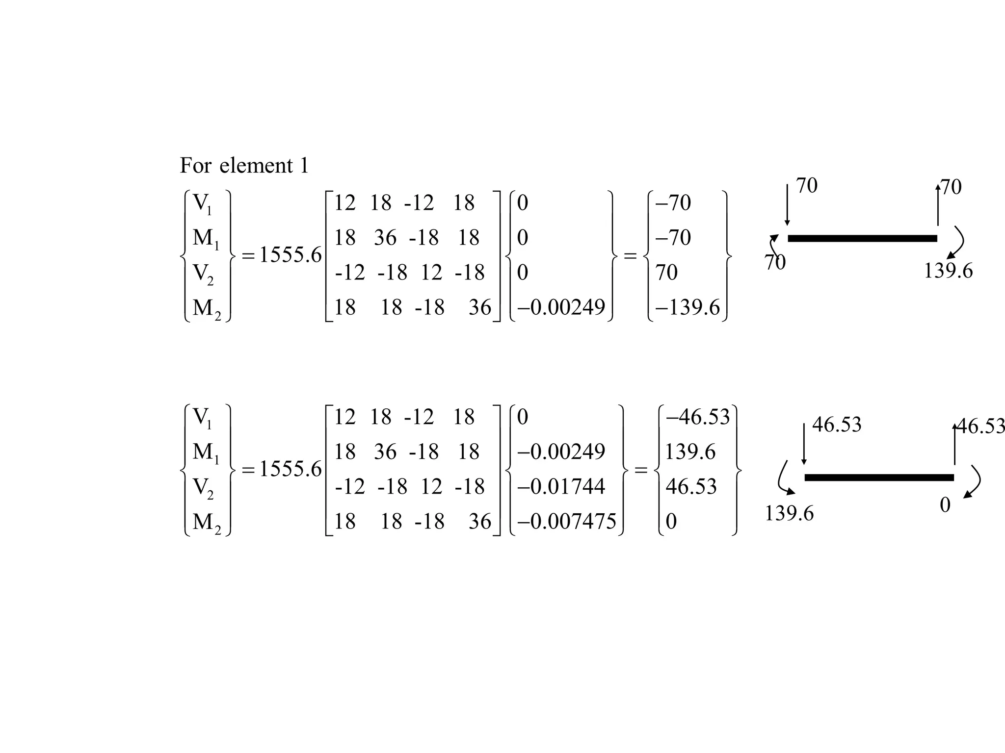
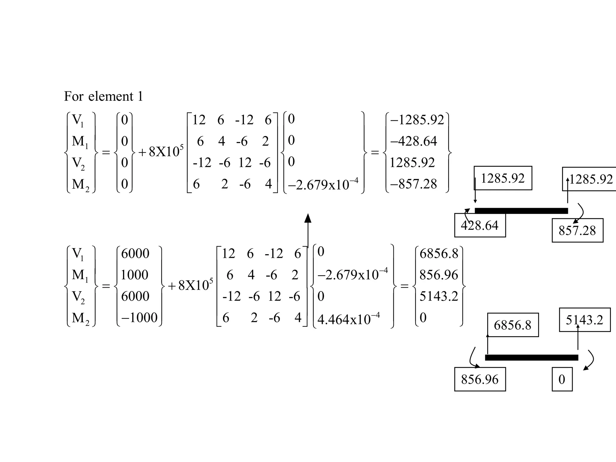
Final member end forces
f k d {FEMS}
−
−
θ −
= θ
θ − −
= = θ
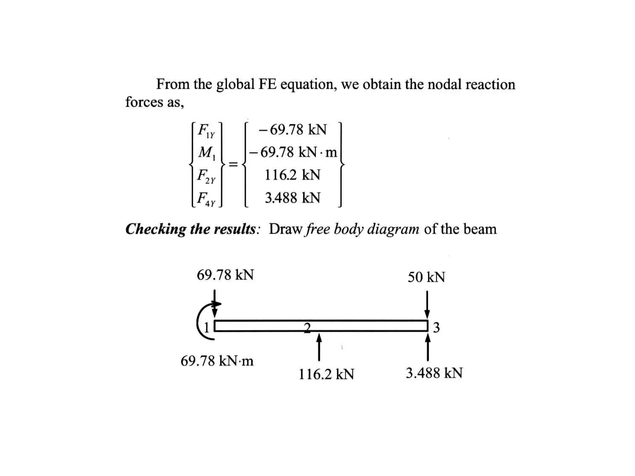
= +](https://image.slidesharecdn.com/2dbeamelementwithcombinedloadingbendingaxialandtorsion-170720044252/75/2d-beam-element-with-combined-loading-bending-axial-and-torsion-22-2048.jpg)
![7/15/2016 26
1
1
2
2
3
3
F 1875 3750 -1875 3750
M 3750 10000 -3750 5000
F -1875 -3750 1875+555.56 -3750+1666.67 -555.56 1666.67
M
F
M
=
3750 5000 -3750+1666.67 10000+6666.67 -1666.67 3333.33
-555.56 -1666.67 555.56 -1666.67
1666.67
1
1
2
2
3
3
1 1 2 3
2 3
v
v
v
3333.332 -1666.67 6666.67
Boundary condition
v , ,v , 0
Loading Condition
M 50; F 60
16666.67 -1666.67
-1666.67 555.56
θ
θ
θ
θ θ =
=− =−
{ } [ ]{ }
2
3
2
3
50
v 60
555.56 1666.67 50 0.0197141
v 1666.67 16666.67 60 0.167146481481.5
Final member end forces
f k d {FEMS}
θ −
=
−
θ − −
= − −
= +](https://image.slidesharecdn.com/2dbeamelementwithcombinedloadingbendingaxialandtorsion-170720044252/75/2d-beam-element-with-combined-loading-bending-axial-and-torsion-26-2048.jpg)

![{ } [ ]{ }
If f ' member end forces in local coordinates then
f' k' q'=
3 3 3 3
3 3 3 3
3 3 3 3
3 3 3 3
AE AE
0 0 0 0
L L
12EI 6EI 12EI 6EI
0 0
L L L L
6EI 4EI 6EI 2EI
0 0
L L L L[k]
AE AE
0 0 0 0
L L
12EI 6EI 12EI 6EI
0 0
L L L L
6EI 2EI 6EI 4EI
0 0
L L L L
−
−
−
=
−
− − −
−
](https://image.slidesharecdn.com/2dbeamelementwithcombinedloadingbendingaxialandtorsion-170720044252/75/2d-beam-element-with-combined-loading-bending-axial-and-torsion-29-2048.jpg)
![{ } { }
[ ] [ ] [ ][ ]T
using conditions q' [L]{q}; and f' [L]{f}
Stiffness matrix for an arbitrarily oriented beam element is given by
k L k' L
= =
=](https://image.slidesharecdn.com/2dbeamelementwithcombinedloadingbendingaxialandtorsion-170720044252/75/2d-beam-element-with-combined-loading-bending-axial-and-torsion-31-2048.jpg)
![{ } [ ]{ }
If f ' member end forces in local coordinates then
f' k' q'=
3 3 3 3
3 3 3 3
3 3 3 3
3 3 3 3
GJ GJ
0 0 0 0
L L
12EI 6EI 12EI 6EI
0 0
L L L L
6EI 4EI 6EI 2EI
0 0
L L L L
GJ GJ
0 0 0 0
L L
12EI 6EI 12EI 6EI
0 0
L L L L
6EI 2EI 6EI 4EI
0 0
L L L L
−
−
−
−
− − −
−
](https://image.slidesharecdn.com/2dbeamelementwithcombinedloadingbendingaxialandtorsion-170720044252/75/2d-beam-element-with-combined-loading-bending-axial-and-torsion-34-2048.jpg)
![[ ]
C 0 -s 0 0 0
0 1 0 0 0 0
-s 0 c 0 0 0
L
0 0 0 c 0 -s
0 0 0 0 1 0
0 0 0 --s 0 c
=
[ ] [ ] [ ][ ]T
k L k' L
=
](https://image.slidesharecdn.com/2dbeamelementwithcombinedloadingbendingaxialandtorsion-170720044252/75/2d-beam-element-with-combined-loading-bending-axial-and-torsion-35-2048.jpg)