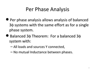
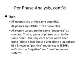
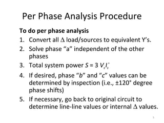
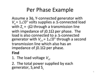
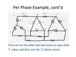
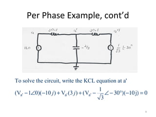
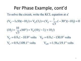
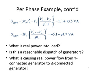
This document provides an overview and summary of key concepts from a lecture on three-phase power system operations and analysis: 1) It introduces the per-phase analysis method which allows analysis of a balanced three-phase system as if it were a single phase by representing loads and sources as wye-connected equivalents and assuming phases are decoupled. 2) It provides an example of using the per-phase analysis method to solve a circuit and determine real and reactive power flows between generators supplying a delta-connected load. 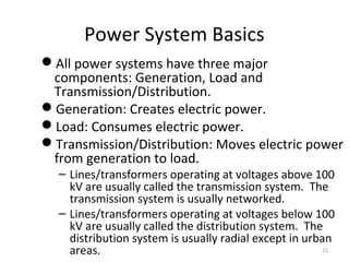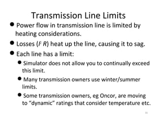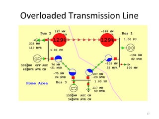3) It discusses basic power system components and operations including generation, load, transmission, distribution of power, and the goal of maintaining real and reactive power balance at all buses.

1. EE369
POWER SYSTEM ANALYSIS
Lecture 3
Three Phase, Power System Operation
Tom Overbye and Ross Baldick
1

2. Reading and Homework
• For lecture 3 read Chapters 1 and 2
• For lectures 4 through 6 read Chapter 4
– we will not be covering sections 4.7, 4.11, and
4.12 in detail,
– We will return to chapter 3 later.
• HW 3 is Problems 2.43, 2.45, 2.46, 2.47, 2.49,
2.50, 2.51, 2.52, 4.2, 4.3, 4.5, 4.7 and Chapter
4 case study questions A through D; due
Thursday 9/17.
2

3. Per Phase Analysis
Per phase analysis allows analysis of balanced
3φ systems with the same effort as for a single
phase system.
Balanced 3φ Theorem: For a balanced 3φ
system with:
– All loads and sources Y connected,
– No mutual Inductance between phases.
3

4. Per Phase Analysis, cont’d
Then
– All neutrals are at the same potential,
– All phases are COMPLETELY decoupled,
– All system values are the same “sequence” as
sources. That is, peaks of phases occur in the
same order. The sequence order we’ve been
using (phase b lags phase a and phase c lags phase
b) is known as “positive” sequence; in EE368L
we’ll discuss “negative” and “zero” sequence
systems.
4

5. Per Phase Analysis Procedure
To do per phase analysis
1. Convert all ∆ load/sources to equivalent Y’s.
2. Solve phase “a” independent of the other
phases
3. Total system power S = 3 VaIa
*
4. If desired, phase “b” and “c” values can be
determined by inspection (i.e., ±120° degree
phase shifts)
5. If necessary, go back to original circuit to
determine line-line values or internal ∆ values.
5

6. Per Phase Example
Assume a 3φ, Y-connected generator with
Van= 1∠0° volts supplies a ∆-connected load
with Z∆ = -jΩ through a transmission line
with impedance of j0.1Ω per phase. The
load is also connected to a ∆-connected
generator with Va’’b’’= 1∠0° through a second
transmission line which also has an
impedance of j0.1Ω per phase.
Find
1. The load voltage Va’b’
2. The total power supplied by each
generator, SYand S∆
6

7. Per Phase Example, cont’d
First convert the delta load and source to equivalent
Y values and draw just the "a" phase circuit
7
+-

8. Per Phase Example, cont’d
a' a' a'
To solve the circuit, write the KCL equation at a'
1
(V 1 0)( 10 ) V (3 ) (V j
3
j j− ∠ − + + − ∠ − 30°)(−10 ) = 0
8

9. Per Phase Example, cont’d
a' a' a'
a'
a' b'
c' a'b'
To solve the circuit, write the KCL equation at a'
1
(V 1 0)( 10 ) V (3 ) (V j
3
10
(10 60 ) V (10 3 10 )
3
V 0.9 volts V 0.9 volts
V 0.9 volts V 1.56
j j
j j j j
− ∠ − + + − ∠ − 30°)(−10 ) = 0
+ ∠ ° = − +
= ∠ −10.9° = ∠ −130.9°
= ∠109.1° = ∠19 volts.1°
9

10. Per Phase Example, cont’d
• What is real power into load?
• Is this a reasonable dispatch of generators?
• What is causing real power flow from Y-
connected generator to ∆-connected
generator? 10
*
* '
ygen
*
'' '
''
S 3 5.1 3.5 VA
0.1
3 5.1 4.7 VA
0.1
a a
a a a
a a
gen a
V V
V I V j
j
V V
S V j
j
∆
 −
= = = + ÷
 
 −
= = − − ÷
 

11. Power System Operations Overview
Goal is to provide an intuitive feel for power
system operation
Emphasis will be on the impact of the
transmission system
Introduce basic power flow concepts
through small system examples
11

12. Power System Basics
All power systems have three major
components: Generation, Load and
Transmission/Distribution.
Generation: Creates electric power.
Load: Consumes electric power.
Transmission/Distribution: Moves electric power
from generation to load.
– Lines/transformers operating at voltages above 100
kV are usually called the transmission system. The
transmission system is usually networked.
– Lines/transformers operating at voltages below 100
kV are usually called the distribution system. The
distribution system is usually radial except in urban
areas. 12

13. Small PowerWorld Simulator Case
Bus 2 Bus 1
Bus 3Home Area
204 MW
102 MVR
150 MW
150 MW
37 MVR
116 MVR
102 MW
51 MVR
1.00 PU
-20 MW
4 MVR
20 MW
-4 MVR
-34 MW
10 MVR
34 MW
-10 MVR
14 MW
-4 MVR
-14 MW
4 MVR
1.00 PU
1.00 PU
106 MW
0 MVR
100 MW
AGC ON
AVR ON
AGC ON
AVR ON
Load with
green
arrows
indicating
amount
of MW
flow
Used
to control
output of
generator
Direction of arrow on line is used to
Indicate direction of real power (MW) flow
Note real
and reactive
power
balance at
each bus13
Closed circuit breaker
is shown as red box
Pie chart and numbers show
real and reactive power flow
Voltage
shown in
normalized
“per unit”
values

14. Power Balance Constraints
Power flow refers to how the power is
moving through the system.
At all times in the simulation the total power
flowing into any bus MUST be zero!
This is due to Kirchhoff’s current law. It can
not be repealed or modified!
Power is lost in the transmission system:
If losses are small, the sending and receiving end
power may appear the same when shown to two
significant figures. 14

15. Basic Power Control
Opening a circuit breaker causes the power
flow to (nearly) instantaneously change.
Other ways to directly control power flow in
an AC transmission line require either power
electronics, or transformers, or both:
See “phase shifting transformers” in lecture 10.
By changing generation (or, in principle, by
changing load) we can indirectly change this
flow.
15

16. Transmission Line Limits
Power flow in transmission line is limited by
heating considerations.
Losses (I2
R) heat up the line, causing it to sag.
Each line has a limit:
Simulator does not allow you to continually exceed
this limit.
Many transmission owners use winter/summer
limits.
Some transmission owners, eg Oncor, are moving
to “dynamic” ratings that consider temperature etc.
16

17. Overloaded Transmission Line
Bus 2 Bus 1
Bus 3Home Area
235 MW
117 MVR
502 MW
150 MW
54 MVR
68 MVR
117 MW
59 MVR
1.00 PU
192 MW
-29 MVR
-188 MW
47 MVR
76 MW
-21 MVR
-75 MW
24 MVR
107 MW
-29 MVR
-105 MW
35 MVR
1.00 PU
1.00 PU
-194 MW
82 MVR
129% 129%
100 MW
OFF AGC
AVR ON
AGC ON
AVR ON
17