The document describes the use of the QIIME2 software suite for analyzing 16S rRNA gene sequences to generate taxonomic profiles and community diversity insights from microbial data. It outlines the entire process from raw data transformation to visualizations, detailing necessary data formatting, the software setup, and specific commands for various analytical steps, such as denoising, taxonomic classification, and phylogenetic analysis. The chapter serves as a comprehensive guide, also providing access to example data and scripts for practical application.

1. Chapter 8
16S rRNA Gene Analysis with QIIME2
Michael Hall and Robert G. Beiko
Abstract
Microbial marker-gene sequence data can be used to generate comprehensive taxonomic profiles of the
microorganisms present in a given community and for other community diversity analyses. The process of
going from raw gene sequences to taxonomic profiles or diversity measures involves a series of data
transformations performed by numerous computational tools. This includes tools for sequence quality
checking, denoising, taxonomic classification, alignment, and phylogenetic tree building. In this chapter,
we demonstrate how the Quantitative Insights Into Microbial Ecology version 2 (QIIME2) software suite
can simplify 16S rRNA marker-gene analysis. We walk through an example data set extracted from the guts
of bumblebees in order to show how QIIME2 can transform raw sequences into taxonomic bar plots,
phylogenetic trees, principal co-ordinates analyses, and other visualizations of microbial diversity.
Key words Microbial ecology, Marker gene, 16S rRNA gene, QIIME, Bioinformatics
1 Introduction
Molecular techniques give us the ability to characterize microor-
ganisms and gain insight into the important biological processes
that they drive. Modern high-throughput methods allow for the
interrogation of entire communities of microorganisms in parallel.
One such method is marker gene analysis. In this type of microbial
community analysis, a phylogenetically informative and universal
gene (or gene fragment) is isolated and amplified with the polymer-
ase chain reaction (PCR). The amplified gene product is sequenced
and the variation within the gene sequences is exploited to predict
the taxonomic groups that are present in a sample, their relative
abundances, and community-diversity measures.
These community descriptors are generated by a series of
computational transformations of the original sequence data.
Some of these transformations, such as sequence quality filtering,
sequence alignments, and phylogeny building, are common bioin-
formatic tasks that can be accomplished with more general tools.
Other transformations, such as taxonomic classification, or the
Robert G. Beiko et al. (eds.), Microbiome Analysis: Methods and Protocols, Methods in Molecular Biology, vol. 1849,
https://doi.org/10.1007/978-1-4939-8728-3_8, © Springer Science+Business Media, LLC, part of Springer Nature 2018
113

2. quantification of community-profile similarity are more likely to
require databases and tools designed specifically for marker-gene
analyses. Dozens of software tools and dependencies are required
for a complete analysis, written in various programming languages
and with documentation spread across many different locations.
These tools interact with one another in a process workflow, feed-
ing from one to the next. Often, the output format of one step does
not match the input requirements of the next step, so an additional
transformation is required. This can lead to complicated analyses
that are performed with ad-hoc commands and data manipulations
that make analysis replication and data-provenance tracking diffi-
cult or impossible.
This chapter demonstrates a microbial marker-gene analysis
using the Quantitative Insights Into Microbial Ecology version
2 (QIIME2, pronounced “chime two”) software suite [3].
QIIME2 provides a software environment, data standards, and
tool wrappers that allow for seamless interoperability between
tools used for microbial community analysis. We describe a typical
analysis pipeline using QIIME2, and demonstrate how study repli-
cation and data provenance can be simplified with scripting and
QIIME artifacts. This chapter is accompanied by a GitHub reposi-
tory (https:/
/github.com/beiko-lab/mimb_16S) which contains
scripts to download an example data set and process the data
using the marker-gene analysis pipeline described here.
2 Materials
2.1 Sequence Data This protocol requires a marker-gene data set generated from a 16S
rRNA gene fragment and sequenced as paired-end reads on an
Illumina platform. While in principle other genes and sequencing
platforms could be used with QIIME2 and its associated tools, the
default parameters and databases are tuned for the 16S rRNA gene
and Illumina paired-end sequences. Use of sequence data from
other genes or sequencing platforms would necessitate substituting
an appropriate reference sequence set and a critical re-evaluation of
default parameters and models on many steps, but particularly those
associated with sequence denoising and taxonomic classification.
Sequence data should be in FASTQ format and must be named
using the Illumina naming convention. For example, a gzip-
compressed FASTQ file may be called SampleName_S1_L001_
R2_001.fastq.gz, where SampleName is the name of the
sample, S1 indicates the sample number on the sample sheet,
L001 indicates the lane number, R2 indicates that the file contains
the reverse reads (with R1 indicating forward reads), and the last
three numbers are always 001 by convention. The files should
be demultiplexed, which means that there is one FASTQ sequence
file for every sample, and all of the FASTQ files should be placed
114 Michael Hall and Robert G. Beiko

3. into the same directory. This directory should contain only two
other files. The first is metadata.yaml. This is a simple text file
that contains only the text {phred-offset: 33} on a single line
(see Note 1). The second file is named MANIFEST and is a three-
column comma-separated text file with the first column listing the
sample name (matching the FASTQ filename convention), the
second column listing the FASTQ file name, and the third column
listing whether the reads are “forward” or “reverse.” Here are the
first 5 lines of the MANIFEST file from the example data set:
sample-id,filename,direction
SRR3202913,SRR3202913_S0_L001_R1_001.fastq.gz,forward
SRR3202913,SRR3202913_S0_L001_R2_001.fastq.gz,reverse
SRR3202914,SRR3202914_S0_L001_R1_001.fastq.gz,forward
SRR3202914,SRR3202914_S0_L001_R2_001.fastq.gz,reverse
To import a directory of sequence files into QIIME, the direc-
tory must contain all of the FASTQ files, a metadata.yml file, and
a complete MANIFEST file listing each of the FASTQ files in the
directory. Subheading 3.1 describes the import process.
2.2 Sample Metadata Sample metadata is stored in a tab-separated text file. Each row
represents a sample, and each column represents a metadata cate-
gory. The first line is a header that contains the metadata category
names. These cannot contain special characters and must be
unique. The first column is used for sample names and must use
the same names as in the sample-id column of the MANIFEST file.
The QIIME developers host a browser-based metadata validation
tool, Keemei (https:/
/keemei.qiime2.org/), that checks for correct
formatting and helps identify any errors in the metadata file
[16]. Metadata files used in QIIME1 analyses are compatible with
QIIME2 and can be used without modification.
2.3 Software For this computational pipeline, we will be using the 2018.2 distri-
bution of the QIIME2 software suite. The installation process has
been significantly simplified over previous iterations of QIIME.
The entire package, including all dependencies and tools, can be
automatically installed with the Anaconda/Miniconda package and
environment manager (available at https:/
/anaconda.org/). The
QIIME software is placed in a virtual environment so that it does
not interfere or conflict with any existing software on the system.
Once installed, the environment must be activated with the com-
mand source activate qiime2-2018.2, giving access to
QIIME as well as the tools that it wraps. It is important to note
that changes to the command line interface can occur between
QIIME2 releases and with plugin updates. The companion GitHub
repository will list any necessary changes to the protocol that may
arise over time.
16S rRNA Gene Analysis with QIIME2 115

4. 3 Methods
3.1 Import Data In QIIME2, there are two main input/output file types: QIIME
artifacts (.qza) and QIIME visualizations (.qzv). QIIME artifacts
encapsulate the set of (potentially heterogeneous) data that results
from a given step in the pipeline. The artifact also contains a variety
of metadata including software versions, command parameters,
timestamps, and run times. QIIME visualization files are analysis
endpoints that contain the data to be visualized along with the code
required to visualize it. Visualizations can be launched in a web
browser with the qiime tools view command, and many feature
interactive elements that facilitate data exploration. Data can be
extracted from .qza or .qzv files using the qiime tools extract
command (see Note 2).
If the sequences are in a directory named sequence_data
(along with a metadata.yml and MANIFEST file, as described in
Subheading 2.1), then the command to import these sequences
into a QIIME artifact is:
qiime tools import --type
’SampleData[PairedEndSequencesWithQuality]’ --input-path
sequence_data --output-path reads
The data type is specified as SampleData[PairedEndSe-
quencesWithQuality]. This is QIIME’s way of indicating that
there are paired forward/reverse FASTQ sequence files for each
sample (see Note 3). An output artifact named reads.qza will be
created, and this file will contain a copy of each of the sequence data
files (see Note 4).
3.2 Visualize
Sequence Quality
The quality profile of sequences can vary depending on sequencing
platform, chemistry, target gene, and many other experimental
variables. The sequence qualities inform the choices for some of
the sequence-processing parameters, such as the truncation para-
meters of the DADA2 denoising step [2]. QIIME includes an
interactive sequence quality plot, available in the “q2-demux” plu-
gin. The following command will sample 10,000 sequences at
random and plot box plots of the qualities at each base position:
qiime demux summarize --p-n 10000 --i-data reads.qza
--o-visualization qual_viz
The plots, contained within a QIIME visualization .qzv file,
can be viewed in a web browser by providing the .qzv file as an
argument to the qiime tools view command. The sample size
should be set sufficiently high to ensure an accurate representation
of the qualities, but the run time of this command will increase with
the sample size.
116 Michael Hall and Robert G. Beiko

5. Since the reads.qza file was created from paired-end reads,
the visualization will automatically display the quality distributions
for a random sample of both the forward and reverse sequences.
With Illumina paired-end data it is expected for there to be a
decrease in the quality at the higher base positions. The point at
which the quality begins to decrease should inform the truncation
parameter used in the subsequent sequence denoising step. The
truncation value is provided separately for forward and reverse
sequence reads, so it is important to note where the quality decrease
occurs for both sets.
3.3 Denoise
Sequences With
DADA2
As an alternative to OTU clustering at a defined sequence-identity
cut-off (e.g., 97%), QIIME2 offers Illumina sequence denoising via
DADA2 [2]. The qiime dada2 denoise-paired will both
merge and denoise paired-end reads. The command has two
required parameters: --p-trunc-len-f indicates the position at
which the forward sequence will be truncated and --p-trunc-
len-r indicates the position at which the reverse read will be
truncated. Optional parameters include --p-max-ee which con-
trols the maximum number of expected errors in a sequence before
it is discarded (default is 2), and --p-truncq which truncates the
sequence after the first position that has a quality score equal to or
less than the provided value (default is 2). DADA2 requires the
primers to be removed from the data to prevent false positive
detection of chimeras as a result of degeneracy in the primers. If
primers are present in the input sequence files, the optional --p-
trim-left-f and --p-trim-left-r parameters can be set to
the length of the primer sequences in order to remove them before
denoising. The denoising process outputs two artifacts: a table file
and a representative sequence file. The table file can be exported to
the Biological Observation Matrix (BIOM) file format (an HDF5-
based standard) using the qiime tools export command for use
in other utilities [11]. The representative sequence file contains the
denoised sequences, while the table file maps each of the sequences
onto their denoised parent sequence.
3.4 Filter Sequence
Table
After denoising with DADA2, many reads may have been excluded
because they could not be merged or were rejected during chimera
detection. You may wish to exclude any samples that have signifi-
cantly fewer sequences than the majority. The qiime feature-
table summarize command produces a visualization file that
shows the spread of sequence depths across the samples. Use this
visualization to identify a lower bound on the sequence depth and
(if desired) filter out low sequence depth samples with the qiime
feature-table filter-samples command with the --p-
min-frequency parameter.
16S rRNA Gene Analysis with QIIME2 117

6. 3.5 Taxonomic
Classification
The QIIME2 software leverages the machine learning Python
library scikit-learn to classify sequences [14]. A reference set can
be used to train a naı̈ve Bayes classifier which can be saved as a
QIIME2 artifact for later re-use. This avoids re-training the classi-
fier between runs, decreasing the overall run time. The QIIME2
project provides a pre-trained naı̈ve Bayes classifier artifact trained
against Greengenes (13_8 revision) trimmed to contain only the V4
hypervariable region and pre-clustered at 99% sequence identity
[12]. To train a naı̈ve Bayes classifier on a different set of reference
sequences, use the qiime feature-classifier fit-classi-
fier-naive-bayes command. Other pre-trained artifacts are
available on the QIIME2 website (https:/
/docs.qiime2.org/).
Once an appropriate classifier artifact has been created or obtained,
use the qiime feature-classifier classify command to
generate the classification results.
3.6 Visualize
Taxonomic
Classifications
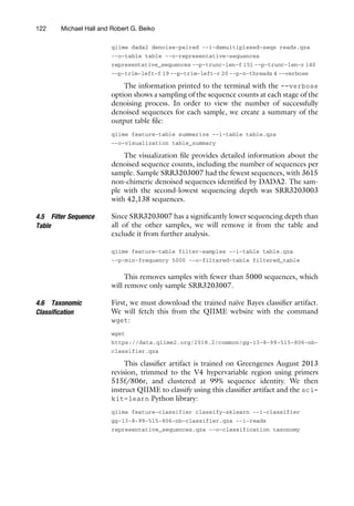
The taxonomic profiles of each sample can be visualized using the
qiime taxa barplot command. This generates an interactive bar
plot of the taxa present in the samples, as determined by the
taxonomic classification algorithm and reference sequence set
used earlier. Bars can be aggregated at the desired taxonomic level
and sorted by abundance of a specific taxonomic group or by
metadata groupings. Color schemes can also be changed interac-
tively, and plots and legends can be saved in vector graphic format.
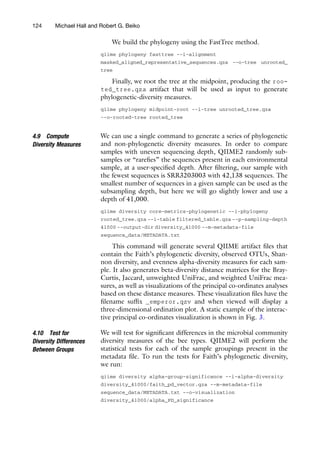
3.7 Build Phylogeny A phylogenetic tree must be created in order to generate phyloge-
netic diversity measures such as unweighted and weighted UniFrac
[9, 10] or Faith’s phylogenetic diversity (PD) [7]. The process is split
into four steps: multiple sequence alignment, masking, tree building,
and rooting. QIIME2 uses MAFFT for the multiple sequence align-
ment via the qiime alignment mafft command [8]. The masking
stage will remove alignment positions that do not contain enough
conservation to provide meaningful information (default 40%) and
can also be set to remove positions that are mostly gaps. The qiime
alignment mask command provides this functionality. The tree
building stage relies on FastTree (see Note 5) and can be invoked
with qiime phylogeny fasttree [15]. The final step, rooting,
takes the unrooted tree output by FastTree and roots it at the mid-
point of the two leaves that are the furthest from one another. This is
done using the qiimephylogeny midpoint-root command. The
end result is a rooted tree artifact file that can be used as input to
generate phylogenetic diversity measures.
3.8 Compute
Diversity Measures
An array of alpha- and beta-diversity measures can be generated
with a single command with QIIME2. The qiime diversity
core-metrics-phylogenetic command will produce both
phylogenetic and non-phylogenetic diversity measures, as well as
alpha- and beta-diversity measures. As input, this command
118 Michael Hall and Robert G. Beiko

7. requires a sequence/OTU table, a phylogenetic tree, and a sam-
pling depth for random subsampling. A good value for the sam-
pling depth is the number of sequences contained in the sample
with the fewest sequences. It can be found by visualizing the
table_summary_output.qzv file from the qiime feature-
table summarize command. The qiime diversity core-
metrics-phylogenetic command generates Faith’s phyloge-
netic diversity, Shannon diversity, evenness, and observed OTUs
(see Note 6) as alpha-diversity measures and weighted/unweighted
UniFrac, Bray-Curtis, and Jaccard as beta-diversity measures. For
each of the beta-diversity measures, QIIME2 automatically gener-
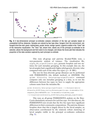
ates principal co-ordinates analysis visualizations. These are three-
dimensional visualizations of the high-dimensional pairwise dis-
tance (or dissimilarity) matrices. These plots allow the researcher
to identify groupings of similar samples at a glance.
3.9 Test for Diversity
Differences Between
Groups
We can test for significant differences between different sample
groups using the qiime diversity alpha-group-signifi-
cance and qiime diversity beta-group-significance
commands. The alpha-diversity group significance command cre-
ates boxplots of the alpha-diversity values and significant differ-
ences between groups are assessed with the Kruskal-Wallis test.
The beta-diversity command uses boxplots to visualize the distance
between samples aggregated by groups specified in the metadata
table file. Significant differences are assessed using a PERMANOVA
analysis [1] or optionally with ANOSIM [5].
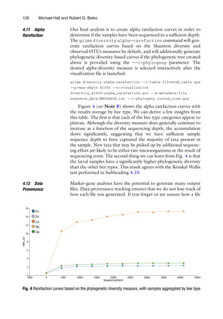
3.10 Alpha
Rarefaction
An alpha rarefaction analysis is used to determine if an environment
has been sequenced to a sufficient depth. This is done by randomly
subsampling the data at a series of sequence depths and plotting the
alpha diversity measures computed from the random subsamples as
a function of the sequencing depth. A plateau on the rarefaction
curve of a given sample provides evidence that the sample has been
sequenced to a sufficient depth to capture the majority of taxa. Use
the qiime diversity alpha-rarefaction command to gener-
ate the visualization file.
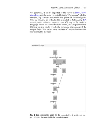
3.11 Data
Provenance
Experimenting with different parameters and plugins can result in
an accumulation of output files. It can be quite easy to lose track of
which commands and parameters were used for which file. Thank-
fully, QIIME2 tracks the provenance of each artifact and visualiza-
tion file. Using the online viewer (https:/
/view.qiime2.org), an
artifact or visualization file can be imported, presenting a prove-
nance tab that shows the history of the file. The viewer lists each of
the parameters used to create the file as well as the run time for the
command and a comprehensive list of plugin and software versions.
This information is provided not only for the imported file, but also
for each of the files that were provided as input, and the input to
16S rRNA Gene Analysis with QIIME2 119

8. those files, and back until the data import command. This means
that each QIIME artifact comes bundled with all the knowledge of
how it was created.
4 Example
4.1 Retrieve Example
Sequence Data
For the example analysis, we will be retrieving data from a recent
study on the gut microbiome of the bumblebee, Bombus pascuorum
[13]. In this study, 106 samples were collected from four different
types of bumblebees. Twenty-four samples were collected from
larvae (La), 47 from nesting bees (Nu), 18 from foragers that
lived in the nest (Fn), 16 from foragers that were collected from
the nearby environment (Fo), and one from the queen (Qu). The
DNA from the microbiota in the midgut and hindgut of each insect
was extracted and amplified using the 515f/806r primer pair (16S
rRNA gene V4 region). DNA sequencing was performed on an
Illumina MiSeq, resulting in a set of paired-end 16S rRNA gene
fragment sequences with an insert size of approximately 254 bp in
length.
The data were deposited in the European Bioinformatics Insti-
tute Short Read Archive (EBI SRA) at project accession
PRJNA313530. The GitHub repository that accompanies this
chapter (https:/
/github.com/beiko-lab/mimb_16S) contains a
BASH script named fetchFastq.sh. This script automatically
downloads the raw FASTQ files and sample metadata from the
EBI SRA.
4.2 Import Data The fetchFastq.sh script creates a directory named sequen-
ce_data/import_to_qiime/ that contains the forward and
reverse FASTQ data files, the MANIFEST file, and the metadata.
yml file. While in the directory containing the fetchFastq.sh
script, the following command will import the FASTQ files into a
QIIME artifact named reads.qza:
qiime tools import --type
’SampleData[PairedEndSequencesWithQuality]’ --input-path
sequence_data/import_to_qiime --output-path reads
4.3 Visualize
Sequence Quality
To generate visualizations of the sequence qualities, we run the
command:
qiime demux summarize --p-n 10000 --i-data reads.qza
--o-visualization qual_viz
Next, the command qiime tools view qual_viz.qzv will
launch the visualization in a web browser. Figure 1 shows the
quality profile across a sample of 10,000 reverse reads. The quality
120 Michael Hall and Robert G. Beiko

9. scores begin slightly lower, which is expected from the bases that
belong to the primer sequences (see Note 7). We will be removing
the primer sequences at the denoising stage. While the median
quality scores remain fairly stable, the variance of the quality scores
increases around position 130. We will trim some of the bases at the
50
end of the reverse reads during the denoising stage.
4.4 Denoise
Sequences With
DADA2
The example sequence data are 2 151 bp paired-end reads from
an Illumina MiSeq using the 515f/806r primer set [4]. The quality
plots (e.g., Fig. 1) indicate that the primers should be trimmed.
The forward primer is 19 bp in length and the reverse primer is
20 bp in length, informing our choice for the parameters --p-
trim-left-f and --p-trim-left-r, respectively. We see an
increase in the variance of the quality scores for the reverse reads,
so we will truncate the reverse reads at position 140. We will not
truncate the forward reads, as the same dramatic increase in quality
variance is not observed. Therefore, the --p-trunc-len-f
parameter will be set to 151, and the --p-trunc-len-r parame-
ter will be set to 140. At an average amplicon length of 254 bp,
trimming the reverse reads by 11 bp would leave an average of
37 bp of overlap. This is sufficient for DADA2, which requires a
minimum of 20 bp of overlap for the read merging step. Using --
p-n-threads 4 allows the program to perform parallel computa-
tions on 4 threads, and the --verbose option displays the
DADA2 progress in the terminal.
Fig. 1 Quality score box plots sampled from 10,000 random reverse reads
16S rRNA Gene Analysis with QIIME2 121

10. qiime dada2 denoise-paired --i-demultiplexed-seqs reads.qza
--o-table table --o-representative-sequences
representative_sequences --p-trunc-len-f 151 --p-trunc-len-r 140
--p-trim-left-f 19 --p-trim-left-r 20 --p-n-threads 4 --verbose
The information printed to the terminal with the --verbose
option shows a sampling of the sequence counts at each stage of the
denoising process. In order to view the number of successfully
denoised sequences for each sample, we create a summary of the
output table file:
qiime feature-table summarize --i-table table.qza
--o-visualization table_summary
The visualization file provides detailed information about the
denoised sequence counts, including the number of sequences per
sample. Sample SRR3203007 had the fewest sequences, with 3615
non-chimeric denoised sequences identified by DADA2. The sam-
ple with the second-lowest sequencing depth was SRR3203003
with 42,138 sequences.
4.5 Filter Sequence
Table
Since SRR3203007 has a significantly lower sequencing depth than
all of the other samples, we will remove it from the table and
exclude it from further analysis.
qiime feature-table filter-samples --i-table table.qza
--p-min-frequency 5000 --o-filtered-table filtered_table
This removes samples with fewer than 5000 sequences, which
will remove only sample SRR3203007.
4.6 Taxonomic
Classification
First, we must download the trained naı̈ve Bayes classifier artifact.
We will fetch this from the QIIME website with the command
wget:
wget
https://data.qiime2.org/2018.2/common/gg-13-8-99-515-806-nb-
classifier.qza
This classifier artifact is trained on Greengenes August 2013
revision, trimmed to the V4 hypervariable region using primers
515f/806r, and clustered at 99% sequence identity. We then
instruct QIIME to classify using this classifier artifact and the sci-
kit-learn Python library:
qiime feature-classifier classify-sklearn --i-classifier
gg-13-8-99-515-806-nb-classifier.qza --i-reads
representative_sequences.qza --o-classification taxonomy
122 Michael Hall and Robert G. Beiko

11. 4.7 Visualize
Taxonomic
Classifications
QIIME can generate interactive bar plots of the taxonomic profiles.
The profiles can be sorted by metadata categories, so we have to
provide the tab-separated metadata file which was generated by the
data download script. The metadata file for the example data is
located in sequence_data/METADATA.txt.
qiime taxa barplot --i-table filtered_table.qza --i-taxonomy
taxonomy.qza --m-metadata-file sequence_data/METADATA.txt
--o-visualization taxa-bar-plots
The resulting taxa-bar-plots.qzv visualization file can be
launched with the command qiime tools view taxa-bar-
plots.qzv. Figure 2 shows taxonomic profiles sorted by bee_-
type and then by the relative abundance of the phylum
Proteobacteria.
4.8 Build Phylogeny We build a phylogeny based on the 16S rRNA gene fragments in
the four-step process described in Subheading 3.7. First, we align
the denoised sequences with MAFFT.
qiime alignment mafft --i-sequences representative_sequences.qza
--o-alignment aligned_representative_sequences
Next, we mask the uninformative positions.
qiime alignment mask --i-alignment
aligned_representative_sequences.qza --o-masked-alignment
masked_aligned_representative_sequences
Fig. 2 Taxonomic profiles for the bumblebee gut samples at phylum level. Samples are sorted first by bee type
and then by the abundance of the phylum Proteobacteria. Bee types are larval samples (La), nesting bees (Nu),
foragers from the nest (Fn), foragers from the environment (Fo), and the queen (Qu)
16S rRNA Gene Analysis with QIIME2 123

12. We build the phylogeny using the FastTree method.
qiime phylogeny fasttree --i-alignment
masked_aligned_representative_sequences.qza --o-tree unrooted_
tree
Finally, we root the tree at the midpoint, producing the roo-
ted_tree.qza artifact that will be used as input to generate
phylogenetic-diversity measures.
qiime phylogeny midpoint-root --i-tree unrooted_tree.qza
--o-rooted-tree rooted_tree
4.9 Compute
Diversity Measures
We can use a single command to generate a series of phylogenetic
and non-phylogenetic diversity measures. In order to compare
samples with uneven sequencing depth, QIIME2 randomly sub-
samples or “rarefies” the sequences present in each environmental
sample, at a user-specified depth. After filtering, our sample with
the fewest sequences is SRR3203003 with 42,138 sequences. The
smallest number of sequences in a given sample can be used as the
subsampling depth, but here we will go slightly lower and use a
depth of 41,000.
qiime diversity core-metrics-phylogenetic --i-phylogeny
rooted_tree.qza --i-table filtered_table.qza --p-sampling-depth
41000 --output-dir diversity_41000 --m-metadata-file
sequence_data/METADATA.txt
This command will generate several QIIME artifact files that
contain the Faith’s phylogenetic diversity, observed OTUs, Shan-
non diversity, and evenness alpha-diversity measures for each sam-
ple. It also generates beta-diversity distance matrices for the Bray-
Curtis, Jaccard, unweighted UniFrac, and weighted UniFrac mea-
sures, as well as visualizations of the principal co-ordinates analyses
based on these distance measures. These visualization files have the
filename suffix _emperor.qzv and when viewed will display a
three-dimensional ordination plot. A static example of the interac-
tive principal co-ordinates visualization is shown in Fig. 3.
4.10 Test for
Diversity Differences
Between Groups
We will test for significant differences in the microbial community
diversity measures of the bee types. QIIME2 will perform the
statistical tests for each of the sample groupings present in the
metadata file. To run the tests for Faith’s phylogenetic diversity,
we run:
qiime diversity alpha-group-significance --i-alpha-diversity
diversity_41000/faith_pd_vector.qza --m-metadata-file
sequence_data/METADATA.txt --o-visualization
diversity_41000/alpha_PD_significance
124 Michael Hall and Robert G. Beiko

13. This runs all-group and pairwise Kruskal-Wallis tests, a
non-parametric analysis of variance. The visualization file,
alpha_PD_significance.qzv, presents boxplots and test sta-
tistics for each metadata grouping. In this example data set, the
larval samples had a significantly higher phylogenetic diversity value
compared with each of the other bee types (p 0. 001).
The test for beta-diversity group distances can be performed
with PERMANOVA (the default method) or ANOSIM. The
qiime diversity beta-group-significance command
computes only one metadata grouping at a time, so to test the
differences between bee types we have to supply the appropriate
column name from the metadata file:
qiime diversity beta-group-significance --i-distance-matrix
diversity_41000/bray_curtis_distance_matrix.qza --m-metadata-file
sequence_data/METADATA.txt --m-metadata-column bee_type
--o-visualization diversity_41000/beta_bray_beetype_significance
This runs an all-group PERMANOVA analysis on the Bray-
Curtis dissimilarity measures for each bee type. For this data set, the
PERMANOVA test reveals that the five bee types have significant
differences in their community compositions. The pairwise distance
boxplots show that this is largely driven by the larval samples, an
observation corroborated by the relatively robust clustering of
larval samples visible in the principal co-ordinates ordination
(Fig. 3).
Fig. 3 A two-dimensional principal co-ordinates analysis ordination of the bee gut samples based on
unweighted UniFrac distances. Samples are colored by bee type (blue: foragers from the environment, red:
foragers from the nest, green: nesting bees, purple: larvae, orange: queen). Legend is visible in the “Color” tab
of the interactive visualization. The “Axis” tab, shown here, allows any of the principal co-ordinates to be
selected, allows the background and font colors to be changed, and shows the Scree plot that indicates the
proportion of the data variation captured by each principal co-ordinate
16S rRNA Gene Analysis with QIIME2 125

14. 4.11 Alpha
Rarefaction
Our final analysis is to create alpha rarefaction curves in order to
determine if the samples have been sequenced to a sufficient depth.
The qiime diversity alpha-rarefaction command will gen-
erate rarefaction curves based on the Shannon diversity and
observed OTUs measures by default, and will additionally generate
phylogenetic diversity-based curves if the phylogenetic tree created
above is provided using the --i-phylogeny parameter. The
desired alpha-diversity measure is selected interactively after the
visualization file is launched.
qiime diversity alpha-rarefaction --i-table filtered_table.qza
--p-max-depth 41000 --o-visualization
diversity_41000/alpha_rarefaction.qzv --m-metadata-file
sequence_data/METADATA.txt --i-phylogeny rooted_tree.qza
Figure 4 (see Note 8) shows the alpha rarefaction curves with
the results average by bee type. We can derive a few insights from
this table. The first is that each of the bee type categories appear to
plateau. Although the diversity measure does generally continue to
increase as a function of the sequencing depth, the accumulation
slows significantly, suggesting that we have sufficient sample
sequence depth to have captured the majority of taxa present in
the sample. New taxa that may be picked up by additional sequenc-
ing effort are likely to be either rare microorganisms or the result of
sequencing error. The second thing we can learn from Fig. 4 is that
the larval samples have a significantly higher phylogenetic diversity
than the other bee types. This result agrees with the Kruskal-Wallis
test performed in Subheading 4.10.
4.12 Data
Provenance
Marker-gene analyses have the potential to generate many output
files. Data-provenance tracking ensures that we do not lose track of
how each file was generated. If you forget or are unsure how a file
Fig. 4 Rarefaction curves based on the phylogenetic diversity measure, with samples aggregated by bee type
126 Michael Hall and Robert G. Beiko

15. was generated, it can be imported to the viewer at https:/
/view.
qiime2.org and the history is available in the “Provenance” tab. For
example, Fig. 5 shows the provenance graph for the unweighted
UniFrac principal co-ordinates file generated in Subheading 4.9,
unweighted_unifrac_emperor.qzv. Clicking on the circles in
the graph reveals the output file type, format, and unique identifier.
Clicking on the blocks reveals the command that generated the
output file(s). The arrows show the flow of output files from one
step as input to the next.
Fig. 5 Data provenance graph for the unweighted_unifrac_em-
peror.qzv file generated in the example analysis
16S rRNA Gene Analysis with QIIME2 127

16. 5 Notes
1. Most recent Illumina sequence data is produced with the
CASAVA pipeline 1.8+ which uses the PHRED+33 encoding
indicated by the “metadata.yml” text {phred-offset: 33}.
If your FASTQ data was generated by an older version of the
CASAVA pipeline, the qualities will be in PHRED+64 format.
In this case, the “metadata.yml” text should be changed to
{phred-offset: 64}.
2. The .qza and .qzv files are simply re-named ZIP files. The file
extension can be changed from .qza or .qvz to .zip and
extracted with any ZIP file decompression tool on systems
where QIIME is not installed or available, such as
Windows PCs.
3. A list of the data types in QIIME2 (2018.2 distribution) is
available at https:/
/docs.qiime2.org/2018.2/semantic-types/.
Single-end FASTQ files correspond to the data type
“SampleData[SequencesWithQuality].”
4. Preserving copies of the raw input data within an artifact
enhances research reproducibility by allowing the source data
to be easily identified and ensures that the data are more closely
coupled to the analysis. Just keep an eye on your hard drive
usage!
5. The QIIME2 2018.2 distribution comes with FastTree version
2.1.10 compiled with double precision. This mitigates issues
with resolving short branch lengths that could occur when
using the version of FastTree that was distributed with earlier
versions of the QIIME software suite.
6. Even though we are not using the common 97% OTU cluster-
ing approach, the denoised sequences from DADA2 can still be
considered operational taxonomic units, so the name
“observed OTUs” is still appropriate for this diversity measure.
However, to avoid confusion, you may wish to describe the
“observed OTUs” measure as “observed taxa” or “observed
representative sequences.”
7. The lower quality scores at the beginning of each read are
caused by the homogeneity of the primer sequences. This
makes it difficult for the Illumina sequencer to properly identify
clusters of DNA molecules [6].
8. Several of the QIIME visualizations do not have a clear way to
export the plots in high-quality scalable vector graphic (SVG)
format. The alpha rarefaction plot is one such visualization. A
simple screenshot will result in a raster graphic that may have
sufficient resolution for inclusion in a research article. The
New York Times’ SVG Crowbar utility (https:/
/nytimes.
128 Michael Hall and Robert G. Beiko

17. github.io/svg-crowbar/) can be used to extract many of these
plots in SVG format. These files can then be easily manipulated
using Inkscape or similar vector graphic-editing programs.
References
1. Anderson M (2005) PERMANOVA: a FOR-
TRAN computer program for permutational
multivariate analysis of variance, 24th edn.
Department of Statistics, University of Auck-
land, Auckland
2. Callahan BJ, McMurdie PJ, Rosen MJ, Han AW,
Johnson AJA, Holmes SP (2016) DADA2:
high-resolution sample inference from Illumina
amplicon data. Nat Methods 13(7):581
3. Caporaso JG, Kuczynski J, Stombaugh J,
Bittinger K, Bushman FD, Costello EK,
Fierer N, Pena AG, Goodrich JK, Gordon JI
et al (2010) QIIME allows analysis of high-
throughput community sequencing data. Nat
Methods 7(5):335
4. Caporaso JG, Lauber CL, Walters WA, Berg-
Lyons D, Lozupone CA, Turnbaugh PJ,
Fierer N, Knight R (2011) Global patterns of
16S rRNA diversity at a depth of millions of
sequences per sample. Proc Natl Acad Sci USA
108:4516–4522
5. Chapman M, Underwood A (1999) Ecological
patterns in multivariate assemblages: informa-
tion and interpretation of negative values in
ANOSIM tests. Mar Ecol Prog Ser
180:257–265
6. Fadrosh DW, Ma B, Gajer P, Sengamalay N,
Ott S, Brotman RM, Ravel J (2014) An
improved dual-indexing approach for multi-
plexed 16S rRNA gene sequencing on the Illu-
mina MiSeq platform. Microbiome 2(1):6
7. Faith DP (1992) Conservation evaluation and
phylogenetic diversity. Biol Conserv 61
(1):1–10
8. Katoh K, Standley DM (2013) MAFFT multi-
ple sequence alignment software version 7:
improvements in performance and usability.
Mol Biol Evol 30(4):772–780
9. Lozupone C, Knight R (2005) UniFrac: a new
phylogenetic method for comparing microbial
communities. Appl Environ Microb 71
(12):8228–8235
10. Lozupone CA, Hamady M, Kelley ST, Knight
R (2007) Quantitative and qualitative β diver-
sity measures lead to different insights into
factors that structure microbial communities.
Appl Environ Microb 73(5):1576–1585
11. McDonald D, Clemente JC, Kuczynski J, Ride-
out JR, Stombaugh J, Wendel D, Wilke A,
Huse S, Hufnagle J, Meyer F et al (2012) The
Biological Observation Matrix (BIOM) format
or: how I learned to stop worrying and love the
ome-ome. GigaScience 1(1):7
12. McDonald D, Price MN, Goodrich J,
Nawrocki EP, DeSantis TZ, Probst A, Ander-
sen GL, Knight R, Hugenholtz P (2012) An
improved Greengenes taxonomy with explicit
ranks for ecological and evolutionary analyses
of bacteria and archaea. ISME J 6(3):610
13. Parmentier A, Meeus I, Nieuwerburgh F,
Deforce D, Vandamme P, Smagghe G
(2018) A different gut microbial community
between larvae and adults of a wild bumble-
bee nest (Bombus pascuorum). Insect Sci 25
(1):66–74
14. Pedregosa F, Varoquaux G, Gramfort A,
Michel V, Thirion B, Grisel O, Blondel M,
Prettenhofer P, Weiss R, Dubourg V et al
(2011) Scikit-learn: machine learning in
Python. J Mach Learn Res 12
(Oct):2825–2830
15. Price MN, Dehal PS, Arkin AP (2010) Fas-
tTree 2–approximately maximum-likelihood
trees for large alignments. PLoS One 5(3):
e9490
16. Rideout JR, Chase JH, Bolyen E,
Ackermann G, González A, Knight R, Capor-
aso JG (2016) Keemei: cloud-based validation
of tabular bioinformatics file formats in Google
Sheets. GigaScience 5(1):27
16S rRNA Gene Analysis with QIIME2 129