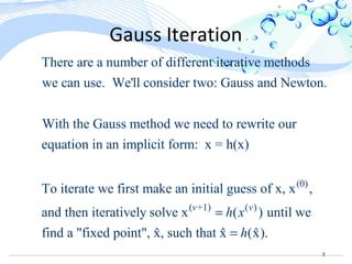
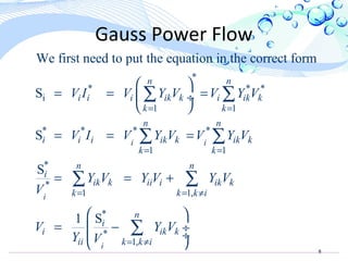
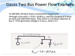
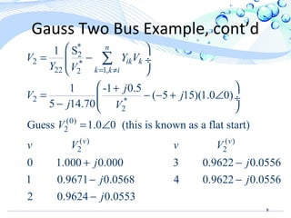
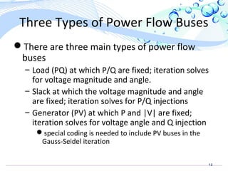
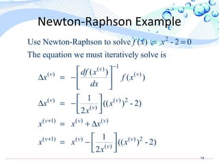
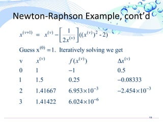
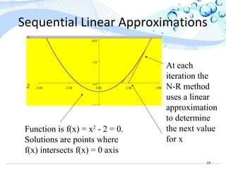
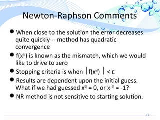
This document provides an overview of the Gauss-Seidel and Newton-Raphson power flow solution methods. It begins by describing the Gauss-Seidel iterative method for solving nonlinear power flow equations using a scalar example. It then discusses applying Gauss-Seidel to vector power flow problems and provides an example of solving a two bus system. The document next describes the Newton-Raphson method, extending it to multidimensional problems using Taylor series approximations and defining the Jacobian matrix. It concludes with brief discussions of advantages and disadvantages of each method.

1. 1
Divyanshu Prakash
B.tech/3rd
Yr./EEE
Mewar University, Chittorgarh

2. 2
Contents
a. Load-Flow analysis
b. Introduction to Newton Raphson Method

3. 3
Gauss Iteration
There are a number of different iterative methods
we can use. We'll consider two: Gauss and Newton.
With the Gauss method we need to rewrite our
equation in an implicit form: x = h(x)
To iterate we fir (0)
( +1) ( )
st make an initial guess of x, x ,
and then iteratively solve x ( ) until we
find a "fixed point", x, such that x (x).ˆ ˆ ˆ
v v
h x
h
=
=

4. 4
Gauss Iteration Example
( 1) ( )
(0)
( ) ( )
Example: Solve - 1 0
1
Let k = 0 and arbitrarily guess x 1 and solve
0 1 5 2.61185
1 2 6 2.61612
2 2.41421 7 2.61744
3 2.55538 8 2.61785
4 2.59805 9 2.61798
v v
v v
x x
x x
k x k x
+
− =
= +
=

5. 5
Stopping Criteria
( ) ( ) ( 1) ( )
A key problem to address is when to stop the
iteration. With the Guass iteration we stop when
with
If x is a scalar this is clear, but if x is a vector we
need to generalize t
v v v v
x x x xε +
∆ < ∆ −@
( )
2
i2
1
he absolute value by using a norm
Two common norms are the Euclidean & infinity
max x
v
j
n
i i
i
x
x
ε
∞
=
∆ <
∆ = ∆ ∆ = ∆∑x x

6. 6
Gauss Power Flow
*
* * *
i
1 1
* * * *
1 1
*
*
1 1,
*
*
1,
We first need to put the equation in the correct form
S
S
S
S1
i i
i
i
n n
i i i ik k i ik k
k k
n n
i i i ik k ik k
k k
n n
i
ik k ii i ik k
k k k i
n
i
i ik k
ii k k i
V I V Y V V Y V
V I V Y V V Y V
Y V Y V Y V
V
V Y V
Y V
= =
= =
= = ≠
= ≠
 
= = = ÷
 
= = =
= = +

= −
∑ ∑
∑ ∑
∑ ∑
∑

 ÷
 ÷
 

7. 7
Gauss Two Bus Power Flow Example
•A 100 MW, 50 Mvar load is connected to a generator
•through a line with z = 0.02 + j0.06 p.u. and line charging of 5 Mvar
on each end (100 MVA base). Also, there is a 25 Mvar capacitor at
bus 2. If the generator voltage is 1.0 p.u., what is V2?
SLoad = 1.0 + j0.5 p.u.

8. 8
Gauss Two Bus Example, cont’d
2
2 bus
bus
22
The unknown is the complex load voltage, V .
To determine V we need to know the .
1
5 15
0.02 0.06
5 14.95 5 15
Hence
5 15 5 14.70
( Note - 15 0.05 0.25)
j
j
j j
j j
B j j j
= −
+
− − + 
=  − + − 
= + +
Y
Y

9. 9
Gauss Two Bus Example, cont’d
*
2
2 *
22 1,2
2 *
2
(0)
2
( ) ( )
2 2
1 S
1 -1 0.5
( 5 15)(1.0 0)
5 14.70
Guess 1.0 0 (this is known as a flat start)
0 1.000 0.000 3 0.9622 0.0556
1 0.9671 0.0568 4 0.9622 0.0556
2 0
n
ik k
k k i
v v
V Y V
Y V
j
V j
j V
V
v V v V
j j
j j
= ≠
 
= − ÷
 
 +
= − − + ∠ ÷
−  
= ∠
+ −
− −
∑
.9624 0.0553j−

10. 10
Gauss Two Bus Example, cont’d
2
* *
1 1 11 1 12 2
1
0.9622 0.0556 0.9638 3.3
Once the voltages are known all other values can
be determined, such as the generator powers and the
line flows
S ( ) 1.023 0.239
In actual units P 102.3 MW
V j
V Y V Y V j
= − = ∠ − °
= + = −
= 1
2
2
, Q 23.9 Mvar
The capacitor is supplying V 25 23.2 Mvar
=
=

11. 11
Slack Bus
In previous example we specified S2 and V1 and
then solved for S1 and V2.
We can not arbitrarily specify S at all buses
because total generation must equal total load +
total losses
We also need an angle reference bus.
To solve these problems we define one bus as
the "slack" bus. This bus has a fixed voltage
magnitude and angle, and a varying real/reactive
power injection.

12. 12
Three Types of Power Flow Buses
There are three main types of power flow
buses
– Load (PQ) at which P/Q are fixed; iteration solves
for voltage magnitude and angle.
– Slack at which the voltage magnitude and angle
are fixed; iteration solves for P/Q injections
– Generator (PV) at which P and |V| are fixed;
iteration solves for voltage angle and Q injection
special coding is needed to include PV buses in the
Gauss-Seidel iteration

13. 13
Gauss-Seidel Advantages
Each iteration is relatively fast (computational
order is proportional to number of branches +
number of buses in the system
Relatively easy to program

14. 14
Gauss-Seidel Disadvantages
Tends to converge relatively slowly, although
this can be improved with acceleration
Has tendency to miss solutions, particularly
on large systems
Tends to diverge on cases with negative
branch reactances (common with
compensated lines)
Need to program using complex numbers

15. 15
Newton-Raphson Algorithm
 Newton-Raphson method is a numerical technique for solving
non-linear equations.
 The second major power flow solution method is the Newton-
Raphson algorithm.
 Key idea behind Newton-Raphson is to use sequential
linearization
General form of problem: Find an x such that
( ) 0ˆf x =

16. 16
Newton-Raphson Method (scalar)
( )
( )
( ) ( )
( )
( ) ( )
2 ( ) 2( )
2
1. For each guess of , , defineˆ
-ˆ
2. Represent ( ) by a Taylor series about ( )ˆ
( )
( ) ( )ˆ
1 ( )
higher order terms
2
v
v v
v
v v
v
v
x x
x x x
f x f x
df x
f x f x x
dx
d f x
x
dx
∆ =
= + ∆ +
+ ∆ +

17. 17
Newton-Raphson Method, cont’d
( )
( ) ( )
( )
1( )
( ) ( )
3. Approximate ( ) by neglecting all termsˆ
except the first two
( )
( ) 0 ( )ˆ
4. Use this linear approximation to solve for
( )
( )
5. Solve for a new estim
v
v v
v
v
v v
f x
df x
f x f x x
dx
x
df x
x f x
dx
−
= ≈ + ∆
∆
 
∆ = − 
 
( 1) ( ) ( )
ate of xˆ
v v v
x x x+
= + ∆

18. 18
Newton-Raphson Example
2
1( )
( ) ( )
( ) ( ) 2
( )
( 1) ( ) ( )
( 1) ( ) ( ) 2
( )
Use Newton-Raphson to solve ( ) - 2 0
The equation we must iteratively solve is
( )
( )
1
(( ) - 2)
2
1
(( ) - 2)
2
v
v v
v v
v
v v v
v v v
v
f x x
df x
x f x
dx
x x
x
x x x
x x x
x
−
+
+
= =
 
∆ = − 
 
 ∆ = −  
= + ∆
 = −   

19. 19
Newton-Raphson Example, cont’d
( 1) ( ) ( ) 2
( )
(0)
( ) ( ) ( )
3 3
6
1
(( ) - 2)
2
Guess x 1. Iteratively solving we get
v ( )
0 1 1 0.5
1 1.5 0.25 0.08333
2 1.41667 6.953 10 2.454 10
3 1.41422 6.024 10
v v v
v
v v v
x x x
x
x f x x
+
− −
−
 = −   
=
∆
−
−
× − ×
×

20. 20
Sequential Linear Approximations
Function is f(x) = x2
- 2 = 0.
Solutions are points where
f(x) intersects f(x) = 0 axis
At each
iteration the
N-R method
uses a linear
approximation
to determine
the next value
for x

21. 21
Newton-Raphson Comments
When close to the solution the error decreases
quite quickly -- method has quadratic
convergence
f(x(v)
) is known as the mismatch, which we would
like to drive to zero
Stopping criteria is when f(x(v)
)  < ε
Results are dependent upon the initial guess.
What if we had guessed x(0)
= 0, or x (0)
= -1?
NR method is not sensitive to starting solution.

22. 22
Multi-Variable Newton-Raphson
1 1
2 2
Next we generalize to the case where is an n-
dimension vector, and ( ) is an n-dimension function
( )
( )
( )
( )
Again define the solution so ( ) 0 andˆ ˆ
n n
x f
x f
x f
   
   
   = =
   
   
   
=
∆ =
x
f x
x
x
x f x
x
x f x
x
M M
ˆ −x x

23. 23
Multi-Variable Case, cont’d
i
1 1
1 1 1 2
1 2
1
n n
n n 1 2
1 2
n
The Taylor series expansion is written for each f ( )
f ( ) f ( )
f ( ) f ( )ˆ
f ( )
higher order terms
f ( ) f ( )
f ( ) f ( )ˆ
f ( )
higher order terms
n
n
n
n
x x
x x
x
x
x x
x x
x
x
∂ ∂
= + ∆ + ∆ +
∂ ∂
∂
∆ +
∂
∂ ∂
= + ∆ + ∆ +
∂ ∂
∂
∆ +
∂
x
x x
x x
x
x x
x x
x
K
M
K

24. 24
Multi-Variable Case, cont’d
1 1 1
1 2
1 1
2 2 2
2 2
1 2
1 2
This can be written more compactly in matrix form
( ) ( ) ( )
( )
( ) ( ) ( )
( )
( )ˆ
( )
( ) ( ) ( )
n
n
n
n n n
n
f f f
x x x
f x
f f f
f x
x x x
f
f f f
x x x
∂ ∂ ∂ 
 ∂ ∂ ∂
  ∆ 
∂ ∂ ∂   ∆   ∂ ∂ ∂= +
  
  
   ∂ ∂ ∂
 
∂ ∂ ∂  
x x x
x
x x x
x
f x
x
x x x
L
L
M
M O O M
L
higher order terms
nx
 
 
 
 
 ∆ 
+
M

25. 25
Jacobian Matrix
1 1 1
1 2
2 2 2
1 2
1 2
The n by n matrix of partial derivatives is known
as the Jacobian matrix, ( )
( ) ( ) ( )
( ) ( ) ( )
( )
( ) ( ) ( )
n
n
n n n
n
f f f
x x x
f f f
x x x
f f f
x x x
∂ ∂ ∂ 
 ∂ ∂ ∂
 
∂ ∂ ∂ 
 ∂ ∂ ∂=
 
 
 ∂ ∂ ∂
 
∂ ∂ ∂  
J x
x x x
x x x
J x
x x x
L
L
M O O M
L

26. 26
References
a. https://www.youtube.com/watch?v=WlQclObEAiA
b. Book: power system engineering/Ngrath &
kothari/1st
edition, 6.6

27. 27