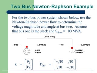
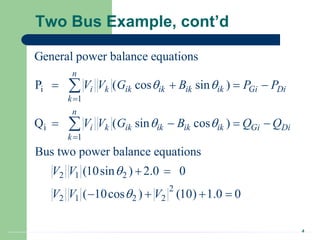
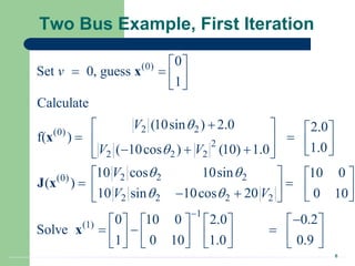
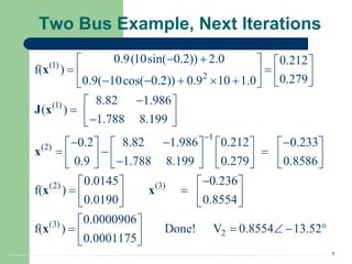
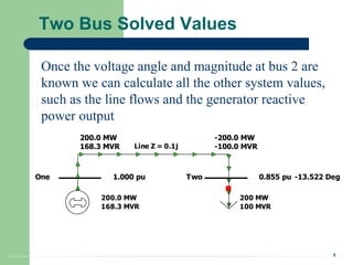
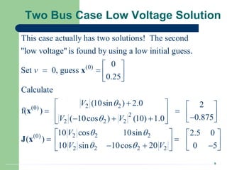
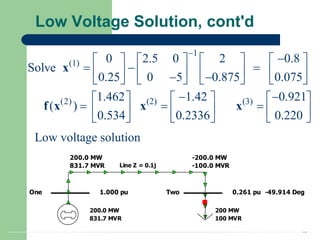
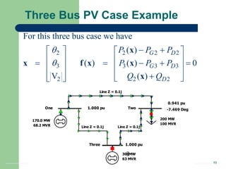
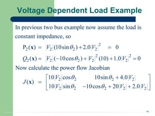
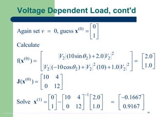
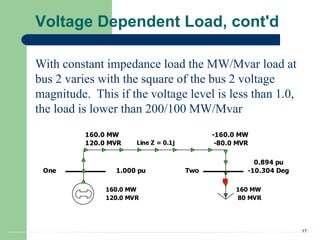
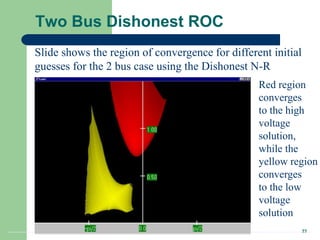
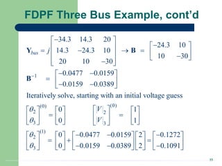
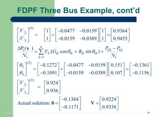
SlideShare a Scribd company logo
1 of 44
Lecture 13
Newton-Raphson Power Flow
Professor Tom Overbye
Department of Electrical and
Computer Engineering
ECE 476
POWER SYSTEM ANALYSIS
1
Announcements
 Homework 6 is 2.38, 6.8, 6.23, 6.28; you should
do it before the exam but need not turn it in.
Answers have been posted.
 First exam is 10/9 in class; closed book, closed
notes, one note sheet and calculators allowed. Last
year’s tests and solutions have been posted.
 Abbott power plant and substation field trip,
Tuesday 10/14 starting at 12:30pm. We’ll meet at
corner of Gregory and Oak streets.
 Be reading Chapter 6; exam covers up through
Section 6.4; we do not explicitly cover 6.1.
2
PV Buses
 Since the voltage magnitude at PV buses is fixed
there is no need to explicitly include these voltages
in x or write the reactive power balance equations
– the reactive power output of the generator varies to
maintain the fixed terminal voltage (within limits)
– optionally these variations/equations can be included by
just writing the explicit voltage constraint for the
generator bus
|Vi | – Vi setpoint = 0
3
Two Bus Newton-Raphson Example
Line Z = 0.1j
One Two
1.000 pu 1.000 pu
200 MW
100 MVR
0 MW
0 MVR
For the two bus power system shown below, use the
Newton-Raphson power flow to determine the
voltage magnitude and angle at bus two. Assume
that bus one is the slack and SBase = 100 MVA.
2
2
10 10
10 10
bus
j j
V j j
 
   
 
   

 
 
x Y
4
Two Bus Example, cont’d
i
1
i
1
2 1 2
2
2 1 2 2
General power balance equations
P ( cos sin )
Q ( sin cos )
Bus two power balance equations
(10sin ) 2.0 0
( 10cos ) (10) 1.0 0
n
i k ik ik ik ik Gi Di
k
n
i k ik ik ik ik Gi Di
k
V V G B P P
V V G B Q Q
V V
V V V
 
 




   
   
 
   


5
Two Bus Example, cont’d
2 2 2
2
2 2 2 2
2 2
2 2
2 2
2 2
2 2 2
2 2 2 2
P ( ) (10sin ) 2.0 0
( ) ( 10cos ) (10) 1.0 0
Now calculate the power flow Jacobian
P ( ) P ( )
( )
Q ( ) Q ( )
10 cos 10sin
10 sin 10cos 20
V
Q V V
V
J
V
V
V V




 
 
  
    
 
 
 
 
 

 
 
 
 
 
 
  
 
 
x
x
x x
x
x x
6
Two Bus Example, First Iteration
(0)
2 2
(0)
2
2 2 2
2 2 2
(0)
2 2 2 2
(1)
0
Set 0, guess
1
Calculate
(10sin ) 2.0 2.0
f( )
1.0
( 10cos ) (10) 1.0
10 cos 10sin 10 0
( )
10 sin 10cos 20 0 10
0 10 0
Solve
1 0 10
v
V
V V
V
V V


 
 
 
   
 

   
 
   
    
 
 
   
 
   
   
 
  
 
 
  
x
x
J x
x
1
2.0 0.2
1.0 0.9


    

     
    
7
Two Bus Example, Next Iterations
(1)
2
(1)
1
(2)
0.9(10sin( 0.2)) 2.0 0.212
f( )
0.279
0.9( 10cos( 0.2)) 0.9 10 1.0
8.82 1.986
( )
1.788 8.199
0.2 8.82 1.986 0.212 0.233
0.9 1.788 8.199 0.279 0.8586
f(

 
   
 
   
      
 

 
  

 
  
       
  
       

       
x
J x
x
(2) (3)
(3)
2
0.0145 0.236
)
0.0190 0.8554
0.0000906
f( ) Done! V 0.8554 13.52
0.0001175

   
 
   
   
 
    
 
 
x x
x
8
Two Bus Solved Values
Line Z = 0.1j
One Two
1.000 pu 0.855 pu
200 MW
100 MVR
200.0 MW
168.3 MVR
-13.522 Deg
200.0 MW
168.3 MVR
-200.0 MW
-100.0 MVR
Once the voltage angle and magnitude at bus 2 are
known we can calculate all the other system values,
such as the line flows and the generator reactive
power output
9
Two Bus Case Low Voltage Solution
(0)
2 2
(0)
2
2 2 2
This case actually has two solutions! The second
"low voltage" is found by using a low initial guess.
0
Set 0, guess
0.25
Calculate
(10sin ) 2.0
f( )
( 10cos ) (10) 1.0
v
V
V V


 
   
 

 
  
  
 
 
x
x
2 2 2
(0)
2 2 2 2
2
0.875
10 cos 10sin 2.5 0
( )
10 sin 10cos 20 0 5
V
V V
 
 
 
  

 
   
 
   
  
 
 
J x
10
Low Voltage Solution, cont'd
1
(1)
(2) (2) (3)
0 2.5 0 2 0.8
Solve
0.25 0 5 0.875 0.075
1.462 1.42 0.921
( )
0.534 0.2336 0.220


       
  
       
 
       
 
     
  
     
     
x
f x x x
Line Z = 0.1j
One Two
1.000 pu 0.261 pu
200 MW
100 MVR
200.0 MW
831.7 MVR
-49.914 Deg
200.0 MW
831.7 MVR
-200.0 MW
-100.0 MVR
Low voltage solution
11
Two Bus Region of Convergence
Slide shows the region of convergence for different initial
guesses of bus 2 angle (x-axis) and magnitude (y-axis)
Red region
converges
to the high
voltage
solution,
while the
yellow region
converges
to the low
voltage
solution
12
Using the Power Flow: Example 1
slack
SLA CK345
SLA CK138
RA Y345
RA Y138
RA Y69
FERNA 69
A
MVA
DEMA R69
BLT 69
BLT 138
BOB138
BOB69
WOLEN69
SHIMKO69
ROGER69
UIUC69
PET E69
HISKY69
T IM69
T IM138
T IM345
PA I69
GROSS69
HA NNA H69
A MA NDA 69
HOMER69
LA UF69
MORO138
LA UF138
HA LE69
PA T T EN69
WEBER69
BUCKY138
SA VOY69
SA VOY138
JO138 JO345
A
MVA
A
MVA
A
MVA
A
MVA
A
MVA
A
MVA
A
MVA
A
MVA
A
MVA
A
MVA
A
MVA
A
MVA
A
MVA
A
MVA
A
MVA
A
MVA
A
MVA
A
MVA
A
MVA
A
MVA
A
MVA
A
MVA
A
MVA
A
MVA
A
MVA
A
MVA
A
MVA
A
MVA
A
MVA
A
MVA
A
MVA
A
MVA
A
MVA
A
MVA
A
MVA
A
MVA
A
MVA
A
MVA
A
MVA
A
MVA
A
MVA
A
MVA
A
MVA
A
MVA
A
MVA
A
MVA
A
MVA
A
MVA
A
MVA
A
MVA
1.02 pu
1.01 pu
1.02 pu
1.03 pu
1.01 pu
1.00 pu
1.00 pu
0.99 pu
1.02 pu
1.01 pu
1.00 pu
1.01 pu
1.01 pu
1.01 pu
1.01 pu
1.02 pu
1.00 pu
1.00 pu
1.02 pu
0.997 pu
0.99 pu
1.00 pu
1.02 pu
1.00 pu
1.01 pu
1.00 pu
1.00 pu 1.00 pu
1.01 pu
1.02 pu
1.02 pu
1.02 pu
1.03 pu
A
MVA
1.02 pu
A
MVA
A
MVA
LYNN138
A
MVA
1.02 pu
A
MVA
1.00 pu
A
MVA
218 MW
54 Mvar
21 MW
7 Mvar
45 MW
12 Mvar
140 MW
45 Mvar
37 MW
13 Mvar
12 MW
5 Mvar
150 MW
0 Mvar
56 MW
13 Mvar
15 MW
5 Mvar
14 MW
2 Mvar
42 MW
2 Mvar
45 MW
0 Mvar
58 MW
36 Mvar
36 MW
10 Mvar
0 MW
0 Mvar
22 MW
15 Mvar
60 MW
12 Mvar
20 MW
30 Mvar
23 MW
7 Mvar
33 MW
13 Mvar
16.0 Mvar 18 MW
5 Mvar
58 MW
40 Mvar
51 MW
15 Mvar
14.3 Mvar
33 MW
10 Mvar
15 MW
3 Mvar
23 MW
6 Mvar 14 MW
3 Mvar
4.8 Mvar
7.2 Mvar
12.8 Mvar
29.0 Mvar
7.4 Mvar
0.0 Mvar
106 MW
8 Mvar
20 MW
8 Mvar
150 MW
0 Mvar
17 MW
3 Mvar
0 MW
0 Mvar
14 MW
4 Mvar
Using
case
from
Example
6.13
13
Three Bus PV Case Example
Line Z = 0.1j
Line Z = 0.1j Line Z = 0.1j
One Two
1.000 pu
0.941 pu
200 MW
100 MVR
170.0 MW
68.2 MVR
-7.469 Deg
Three 1.000 pu
30 MW
63 MVR
2 2 2 2
3 3 3 3
2 2 2
For this three bus case we have
( )
( ) ( ) 0
V ( )
G D
G D
D
P P P
P P P
Q Q


 
   
   
    
   

   
 
 
x
x f x x
x
14
Modeling Voltage Dependent Load
So far we've assumed that the load is independent of
the bus voltage (i.e., constant power). However, the
power flow can be easily extended to include voltage
depedence with both the real and reactive l
Di Di
1
1
oad. This
is done by making P and Q a function of :
( cos sin ) ( ) 0
( sin cos ) ( ) 0
i
n
i k ik ik ik ik Gi Di i
k
n
i k ik ik ik ik Gi Di i
k
V
V V G B P P V
V V G B Q Q V
 
 


   
   


15
Voltage Dependent Load Example
2
2 2 2 2
2 2
2 2 2 2 2
2 2 2 2
In previous two bus example now assume the load is
constant impedance, so
P ( ) (10sin ) 2.0 0
( ) ( 10cos ) (10) 1.0 0
Now calculate the power flow Jacobian
10 cos 10sin 4.0
( )
10
V V
Q V V V
V V
J


 
  
    


x
x
x
2 2 2 2 2
sin 10cos 20 2.0
V V V
 
 
 
  
 
16
Voltage Dependent Load, cont'd
(0)
2
2 2 2
(0)
2 2
2 2 2 2
(0)
1
(1)
0
Again set 0, guess
1
Calculate
(10sin ) 2.0 2.0
f( )
1.0
( 10cos ) (10) 1.0
10 4
( )
0 12
0 10 4 2.0 0.1667
Solve
1 0 12 1.0 0.9167
v
V V
V V V



 
   
 
 
  
 
   
 
 
  
 
 
  
 

      
  
     
     
x
x
J x
x

 
 
17
Voltage Dependent Load, cont'd
Line Z = 0.1j
One Two
1.000 pu
0.894 pu
160 MW
80 MVR
160.0 MW
120.0 MVR
-10.304 Deg
160.0 MW
120.0 MVR
-160.0 MW
-80.0 MVR
With constant impedance load the MW/Mvar load at
bus 2 varies with the square of the bus 2 voltage
magnitude. This if the voltage level is less than 1.0,
the load is lower than 200/100 MW/Mvar
18
Solving Large Power Systems
 The most difficult computational task is inverting the
Jacobian matrix
– inverting a full matrix is an order n3 operation, meaning
the amount of computation increases with the cube of the
size size
– this amount of computation can be decreased substantially
by recognizing that since the Ybus is a sparse matrix, the
Jacobian is also a sparse matrix
– using sparse matrix methods results in a computational
order of about n1.5.
– this is a substantial savings when solving systems with
tens of thousands of buses
19
Newton-Raphson Power Flow
 Advantages
– fast convergence as long as initial guess is close to
solution
– large region of convergence
 Disadvantages
– each iteration takes much longer than a Gauss-Seidel
iteration
– more complicated to code, particularly when
implementing sparse matrix algorithms
 Newton-Raphson algorithm is very common in
power flow analysis
20
Dishonest Newton-Raphson
 Since most of the time in the Newton-Raphson
iteration is spend calculating the inverse of the
Jacobian, one way to speed up the iterations is to
only calculate/inverse the Jacobian occasionally
– known as the “Dishonest” Newton-Raphson
– an extreme example is to only calculate the Jacobian for
the first iteration
( 1) ( ) ( ) -1 ( )
( 1) ( ) (0) -1 ( )
( )
Honest: - ( ) ( )
Dishonest: - ( ) ( )
Both require ( ) for a solution
v v v v
v v v
v






x x J x f x
x x J x f x
f x
21
Dishonest Newton-Raphson Example
2
1
(0)
( ) ( )
( ) ( ) 2
(0)
( 1) ( ) ( ) 2
(0)
Use the Dishonest Newton-Raphson to solve
( ) - 2 0
( )
( )
1
(( ) - 2)
2
1
(( ) - 2)
2
v v
v v
v v v
f x x
df x
x f x
dx
x x
x
x x x
x


 
 
   
 
 
   
 
 
   
 
22
Dishonest N-R Example, cont’d
( 1) ( ) ( ) 2
(0)
(0)
( ) ( )
1
(( ) - 2)
2
Guess x 1. Iteratively solving we get
v (honest) (dishonest)
0 1 1
1 1.5 1.5
2 1.41667 1.375
3 1.41422 1.429
4 1.41422 1.408
v v v
v v
x x x
x
x x
  
   
 

We pay a price
in increased
iterations, but
with decreased
computation
per iteration
23
Two Bus Dishonest ROC
Slide shows the region of convergence for different initial
guesses for the 2 bus case using the Dishonest N-R
Red region
converges
to the high
voltage
solution,
while the
yellow region
converges
to the low
voltage
solution
24
Honest N-R Region of Convergence
Maximum
of 15
iterations
25
Decoupled Power Flow
 The completely Dishonest Newton-Raphson is not
used for power flow analysis. However several
approximations of the Jacobian matrix are used.
 One common method is the decoupled power flow.
In this approach approximations are used to
decouple the real and reactive power equations.
26
Decoupled Power Flow Formulation
( ) ( )
( ) ( )
( )
( )
( ) ( ) ( )
( )
2 2 2
( )
( )
General form of the power flow problem
( )
( )
( )
where
( )
( )
( )
v v
v v
v
v
v v v
v
D G
v
v
n Dn Gn
P P P
P P P
 
 
     

  
 
  
   
  
  
     
 
 
 
 
 
 
 
 
   
 
 
 
P P
θ
θ V P x
f x
Q x
V
Q Q
θ V
x
P x
x
27
Decoupling Approximation
( ) ( )
( )
( ) ( )
( )
( ) ( ) ( )
Usually the off-diagonal matrices, and
are small. Therefore we approximate them as zero:
( )
( )
( )
Then the problem
v v
v
v v
v
v v v
 
 
 

     
 

 
  
   
 
 
  
   
 
 

 
P Q
V θ
P
0
θ P x
θ
f x
Q Q x
V
0
V
1 1
( ) ( )
( )
( ) ( ) ( )
can be decoupled
( ) ( )
v v
v
v v v
 
   
 
       
   
 
   
P Q
θ P x V Q x
θ V
28
Off-diagonal Jacobian Terms
 
 
Justification for Jacobian approximations:
1. Usually r x, therefore
2. Usually is small so sin 0
Therefore
cos sin 0
cos sin 0
ij ij
ij ij
i
i ij ij ij ij
j
i
i j ij ij ij ij
j
G B
V G B
V V G B
 
 
 


  


   

P
V
Q
θ
29
Decoupled N-R Region of Convergence
30
Fast Decoupled Power Flow
 By continuing with our Jacobian approximations we
can actually obtain a reasonable approximation that
is independent of the voltage magnitudes/angles.
 This means the Jacobian need only be built/inverted
once.
 This approach is known as the fast decoupled power
flow (FDPF)
 FDPF uses the same mismatch equations as
standard power flow so it should have same solution
 The FDPF is widely used, particularly when we
only need an approximate solution
31
FDPF Approximations
ij
( ) ( )
( )
( ) 1 1
( ) ( )
bus
The FDPF makes the following approximations:
1. G 0
2. 1
3. sin 0 cos 1
Then
( ) ( )
Where is just the imaginary part of the ,
except the slack bus row/co
i
ij ij
v v
v
v
v v
V
j
 
 


 
 
   
 
P x Q x
θ B V B
V V
B Y G B
lumn are omitted
32
FDPF Three Bus Example
Line Z = j0.07
Line Z = j0.05 Line Z = j0.1
One Two
200 MW
100 MVR
Three 1.000 pu
200 MW
100 MVR
Use the FDPF to solve the following three bus system
34.3 14.3 20
14.3 24.3 10
20 10 30
bus j

 
 
 
 

 
 
Y
33
FDPF Three Bus Example, cont’d
1
(0)
(0)
2 2
3 3
34.3 14.3 20
24.3 10
14.3 24.3 10
10 30
20 10 30
0.0477 0.0159
0.0159 0.0389
Iteratively solve, starting with an initial voltage guess
0 1
0 1
bus j
V
V




 

 
 
     
  
 

 
 
 
 
  
 
 
 
    
 
 
   
 
   
Y B
B
(1)
2
3
0 0.0477 0.0159 2 0.1272
0 0.0159 0.0389 2 0.1091



 
 
  
         
  
         
  
       
 
34
FDPF Three Bus Example, cont’d
(1)
2
3
i
i i
1
(2)
2
3
1 0.0477 0.0159 1 0.9364
1 0.0159 0.0389 1 0.9455
P ( )
( cos sin )
V V
0.1272 0.0477 0.0159
0.1091 0.0159 0.0389
n
Di Gi
k ik ik ik ik
k
V
V
P P
V G B
 



 
         
  
         
 
       
 


  
  
     
 
     
  
   
 

x
(2)
2
3
0.151 0.1361
0.107 0.1156
0.924
0.936
0.1384 0.9224
Actual solution:
0.1171 0.9338
V
V

   

   

   
   

   
 
 

   
 
   

   
θ V
35
FDPF Region of Convergence
36
“DC” Power Flow
 The “DC” power flow makes the most severe
approximations:
– completely ignore reactive power, assume all the voltages
are always 1.0 per unit, ignore line conductance
 This makes the power flow a linear set of equations,
which can be solved directly
1


θ B P
37
Power System Control
 A major problem with power system operation is
the limited capacity of the transmission system
– lines/transformers have limits (usually thermal)
– no direct way of controlling flow down a transmission
line (e.g., there are no valves to close to limit flow)
– open transmission system access associated with industry
restructuring is stressing the system in new ways
 We need to indirectly control transmission line flow
by changing the generator outputs
38
Indirect Transmission Line Control
What we would like to determine is how a change in
generation at bus k affects the power flow on a line
from bus i to bus j.
The assumption is
that the change
in generation is
absorbed by the
slack bus
39
Power Flow Simulation - Before
One way to determine the impact of a generator change
is to compare a before/after power flow.
For example below is a three bus case with an overload
Z for all lines = j0.1
One Two
200 MW
100 MVR
200.0 MW
71.0 MVR
Three 1.000 pu
0 MW
64 MVR
131.9 MW
68.1 MW 68.1 MW
124%
40
Power Flow Simulation - After
Z for all lines = j0.1
Limit for all lines = 150 MVA
One Two
200 MW
100 MVR
105.0 MW
64.3 MVR
Three
1.000 pu
95 MW
64 MVR
101.6 MW
3.4 MW 98.4 MW
92%
100%
Increasing the generation at bus 3 by 95 MW (and hence
decreasing it at bus 1 by a corresponding amount), results
in a 31.3 drop in the MW flow on the line from bus 1 to 2.
41
Analytic Calculation of Sensitivities
 Calculating control sensitivities by repeat power
flow solutions is tedious and would require many
power flow solutions. An alternative approach is to
analytically calculate these values
The power flow from bus i to bus j is
sin( )
So We just need to get
i j i j
ij i j
ij ij
i j ij
ij
ij Gk
V V
P
X X
P
X P
 
 
  

  
   
 

42
Analytic Sensitivities
1
From the fast decoupled power flow we know
( )
So to get the change in due to a change of
generation at bus k, just set ( ) equal to
all zeros except a minus one at position k.
0
1
0

  



  

θ B P x
θ
P x
P Bus k

 
 

 
 
 
 

43
Three Bus Sensitivity Example
line
bus
1
2
3
For the previous three bus case with Z 0.1
20 10 10
20 10
10 20 10
10 20
10 10 20
Hence for a change of generation at bus 3
20 10 0 0.0333
10 20 1 0.0667
j
j





 

 
 
     
  
 

 
 
 
      
 
      
  
    
 
Y B
3 to 1
3 to 2 2 to 1
0.0667 0
Then P 0.667 pu
0.1
P 0.333 pu P 0.333 pu




  
   

More Related Content

Similar to Stability with analysis and psa and load flow.ppt

Load flow study Part-I
Load flow study Part-ILoad flow study Part-I
Load flow study Part-IAsif Jamadar
 
about power system operation and control13197214.ppt
about power system operation and control13197214.pptabout power system operation and control13197214.ppt
about power system operation and control13197214.pptMohammedAhmed66819
 
Newton Raphson method for load flow analysis
Newton Raphson method for load flow analysisNewton Raphson method for load flow analysis
Newton Raphson method for load flow analysisdivyanshuprakashrock
 
UNIT-III complex reactive three phase.ppt
UNIT-III complex reactive three phase.pptUNIT-III complex reactive three phase.ppt
UNIT-III complex reactive three phase.pptAbinaya Saraswathy T
 
ECEN615_Fall2020_Lect4.pptx
ECEN615_Fall2020_Lect4.pptxECEN615_Fall2020_Lect4.pptx
ECEN615_Fall2020_Lect4.pptxPrasenjitDey49
 
Eet3082 binod kumar sahu lecturer_14
Eet3082 binod kumar sahu lecturer_14Eet3082 binod kumar sahu lecturer_14
Eet3082 binod kumar sahu lecturer_14BinodKumarSahu5
 
Eet3082 binod kumar sahu lecturer_14
Eet3082 binod kumar sahu lecturer_14Eet3082 binod kumar sahu lecturer_14
Eet3082 binod kumar sahu lecturer_14BinodKumarSahu5
 
Unit1 And 2 Sample Solutions
Unit1 And 2 Sample SolutionsUnit1 And 2 Sample Solutions
Unit1 And 2 Sample SolutionsAbha Tripathi
 
Resonant circuits
Resonant circuitsResonant circuits
Resonant circuitsarjav patel
 
Unit1 and 2 sample solutions
Unit1 and 2 sample solutionsUnit1 and 2 sample solutions
Unit1 and 2 sample solutionsAbha Tripathi
 
A novel voltage reference without the operational amplifier and resistors
A novel voltage reference without the operational amplifier and resistorsA novel voltage reference without the operational amplifier and resistors
A novel voltage reference without the operational amplifier and resistorsIJRES Journal
 
Analog circuits
Analog circuitsAnalog circuits
Analog circuitsMangi Lal
 
ECE476_2016_Lect 12.pptx
ECE476_2016_Lect 12.pptxECE476_2016_Lect 12.pptx
ECE476_2016_Lect 12.pptxAhmed359095
 

Similar to Stability with analysis and psa and load flow.ppt (20)

Lecture 13
Lecture 13Lecture 13
Lecture 13
 
Lecture 7
Lecture 7Lecture 7
Lecture 7
 
Load flow study Part-I
Load flow study Part-ILoad flow study Part-I
Load flow study Part-I
 
Lecture 2
Lecture 2Lecture 2
Lecture 2
 
about power system operation and control13197214.ppt
about power system operation and control13197214.pptabout power system operation and control13197214.ppt
about power system operation and control13197214.ppt
 
Newton Raphson method for load flow analysis
Newton Raphson method for load flow analysisNewton Raphson method for load flow analysis
Newton Raphson method for load flow analysis
 
Lecture 11
Lecture 11Lecture 11
Lecture 11
 
UNIT-III complex reactive three phase.ppt
UNIT-III complex reactive three phase.pptUNIT-III complex reactive three phase.ppt
UNIT-III complex reactive three phase.ppt
 
Lecture 8
Lecture 8Lecture 8
Lecture 8
 
ECEN615_Fall2020_Lect4.pptx
ECEN615_Fall2020_Lect4.pptxECEN615_Fall2020_Lect4.pptx
ECEN615_Fall2020_Lect4.pptx
 
Eet3082 binod kumar sahu lecturer_14
Eet3082 binod kumar sahu lecturer_14Eet3082 binod kumar sahu lecturer_14
Eet3082 binod kumar sahu lecturer_14
 
Eet3082 binod kumar sahu lecturer_14
Eet3082 binod kumar sahu lecturer_14Eet3082 binod kumar sahu lecturer_14
Eet3082 binod kumar sahu lecturer_14
 
transformer
transformertransformer
transformer
 
Resonant circuits
Resonant circuitsResonant circuits
Resonant circuits
 
Unit1 And 2 Sample Solutions
Unit1 And 2 Sample SolutionsUnit1 And 2 Sample Solutions
Unit1 And 2 Sample Solutions
 
Resonant circuits
Resonant circuitsResonant circuits
Resonant circuits
 
Unit1 and 2 sample solutions
Unit1 and 2 sample solutionsUnit1 and 2 sample solutions
Unit1 and 2 sample solutions
 
A novel voltage reference without the operational amplifier and resistors
A novel voltage reference without the operational amplifier and resistorsA novel voltage reference without the operational amplifier and resistors
A novel voltage reference without the operational amplifier and resistors
 
Analog circuits
Analog circuitsAnalog circuits
Analog circuits
 
ECE476_2016_Lect 12.pptx
ECE476_2016_Lect 12.pptxECE476_2016_Lect 12.pptx
ECE476_2016_Lect 12.pptx
 

Recently uploaded

High Profile Call Girls Nagpur Meera Call 7001035870 Meet With Nagpur Escorts
High Profile Call Girls Nagpur Meera Call 7001035870 Meet With Nagpur EscortsHigh Profile Call Girls Nagpur Meera Call 7001035870 Meet With Nagpur Escorts
High Profile Call Girls Nagpur Meera Call 7001035870 Meet With Nagpur EscortsCall Girls in Nagpur High Profile
 
Processing & Properties of Floor and Wall Tiles.pptx
Processing & Properties of Floor and Wall Tiles.pptxProcessing & Properties of Floor and Wall Tiles.pptx
Processing & Properties of Floor and Wall Tiles.pptxpranjaldaimarysona
 
(ANVI) Koregaon Park Call Girls Just Call 7001035870 [ Cash on Delivery ] Pun...
(ANVI) Koregaon Park Call Girls Just Call 7001035870 [ Cash on Delivery ] Pun...(ANVI) Koregaon Park Call Girls Just Call 7001035870 [ Cash on Delivery ] Pun...
(ANVI) Koregaon Park Call Girls Just Call 7001035870 [ Cash on Delivery ] Pun...ranjana rawat
 
Decoding Kotlin - Your guide to solving the mysterious in Kotlin.pptx
Decoding Kotlin - Your guide to solving the mysterious in Kotlin.pptxDecoding Kotlin - Your guide to solving the mysterious in Kotlin.pptx
Decoding Kotlin - Your guide to solving the mysterious in Kotlin.pptxJoão Esperancinha
 
Call for Papers - African Journal of Biological Sciences, E-ISSN: 2663-2187, ...
Call for Papers - African Journal of Biological Sciences, E-ISSN: 2663-2187, ...Call for Papers - African Journal of Biological Sciences, E-ISSN: 2663-2187, ...
Call for Papers - African Journal of Biological Sciences, E-ISSN: 2663-2187, ...Christo Ananth
 
VIP Call Girls Service Hitech City Hyderabad Call +91-8250192130
VIP Call Girls Service Hitech City Hyderabad Call +91-8250192130VIP Call Girls Service Hitech City Hyderabad Call +91-8250192130
VIP Call Girls Service Hitech City Hyderabad Call +91-8250192130Suhani Kapoor
 
(SHREYA) Chakan Call Girls Just Call 7001035870 [ Cash on Delivery ] Pune Esc...
(SHREYA) Chakan Call Girls Just Call 7001035870 [ Cash on Delivery ] Pune Esc...(SHREYA) Chakan Call Girls Just Call 7001035870 [ Cash on Delivery ] Pune Esc...
(SHREYA) Chakan Call Girls Just Call 7001035870 [ Cash on Delivery ] Pune Esc...ranjana rawat
 
Extrusion Processes and Their Limitations
Extrusion Processes and Their LimitationsExtrusion Processes and Their Limitations
Extrusion Processes and Their Limitations120cr0395
 
The Most Attractive Pune Call Girls Budhwar Peth 8250192130 Will You Miss Thi...
The Most Attractive Pune Call Girls Budhwar Peth 8250192130 Will You Miss Thi...The Most Attractive Pune Call Girls Budhwar Peth 8250192130 Will You Miss Thi...
The Most Attractive Pune Call Girls Budhwar Peth 8250192130 Will You Miss Thi...ranjana rawat
 
VIP Call Girls Service Kondapur Hyderabad Call +91-8250192130
VIP Call Girls Service Kondapur Hyderabad Call +91-8250192130VIP Call Girls Service Kondapur Hyderabad Call +91-8250192130
VIP Call Girls Service Kondapur Hyderabad Call +91-8250192130Suhani Kapoor
 
APPLICATIONS-AC/DC DRIVES-OPERATING CHARACTERISTICS
APPLICATIONS-AC/DC DRIVES-OPERATING CHARACTERISTICSAPPLICATIONS-AC/DC DRIVES-OPERATING CHARACTERISTICS
APPLICATIONS-AC/DC DRIVES-OPERATING CHARACTERISTICSKurinjimalarL3
 
Analog to Digital and Digital to Analog Converter
Analog to Digital and Digital to Analog ConverterAnalog to Digital and Digital to Analog Converter
Analog to Digital and Digital to Analog ConverterAbhinavSharma374939
 
Call Girls Delhi {Jodhpur} 9711199012 high profile service
Call Girls Delhi {Jodhpur} 9711199012 high profile serviceCall Girls Delhi {Jodhpur} 9711199012 high profile service
Call Girls Delhi {Jodhpur} 9711199012 high profile servicerehmti665
 
(ANJALI) Dange Chowk Call Girls Just Call 7001035870 [ Cash on Delivery ] Pun...
(ANJALI) Dange Chowk Call Girls Just Call 7001035870 [ Cash on Delivery ] Pun...(ANJALI) Dange Chowk Call Girls Just Call 7001035870 [ Cash on Delivery ] Pun...
(ANJALI) Dange Chowk Call Girls Just Call 7001035870 [ Cash on Delivery ] Pun...ranjana rawat
 
the ladakh protest in leh ladakh 2024 sonam wangchuk.pptx
the ladakh protest in leh ladakh 2024 sonam wangchuk.pptxthe ladakh protest in leh ladakh 2024 sonam wangchuk.pptx
the ladakh protest in leh ladakh 2024 sonam wangchuk.pptxhumanexperienceaaa
 
Gfe Mayur Vihar Call Girls Service WhatsApp -> 9999965857 Available 24x7 ^ De...
Gfe Mayur Vihar Call Girls Service WhatsApp -> 9999965857 Available 24x7 ^ De...Gfe Mayur Vihar Call Girls Service WhatsApp -> 9999965857 Available 24x7 ^ De...
Gfe Mayur Vihar Call Girls Service WhatsApp -> 9999965857 Available 24x7 ^ De...srsj9000
 
Architect Hassan Khalil Portfolio for 2024
Architect Hassan Khalil Portfolio for 2024Architect Hassan Khalil Portfolio for 2024
Architect Hassan Khalil Portfolio for 2024hassan khalil
 
Call Girls Service Nagpur Tanvi Call 7001035870 Meet With Nagpur Escorts
Call Girls Service Nagpur Tanvi Call 7001035870 Meet With Nagpur EscortsCall Girls Service Nagpur Tanvi Call 7001035870 Meet With Nagpur Escorts
Call Girls Service Nagpur Tanvi Call 7001035870 Meet With Nagpur EscortsCall Girls in Nagpur High Profile
 

Recently uploaded (20)

★ CALL US 9953330565 ( HOT Young Call Girls In Badarpur delhi NCR
★ CALL US 9953330565 ( HOT Young Call Girls In Badarpur delhi NCR★ CALL US 9953330565 ( HOT Young Call Girls In Badarpur delhi NCR
★ CALL US 9953330565 ( HOT Young Call Girls In Badarpur delhi NCR
 
High Profile Call Girls Nagpur Meera Call 7001035870 Meet With Nagpur Escorts
High Profile Call Girls Nagpur Meera Call 7001035870 Meet With Nagpur EscortsHigh Profile Call Girls Nagpur Meera Call 7001035870 Meet With Nagpur Escorts
High Profile Call Girls Nagpur Meera Call 7001035870 Meet With Nagpur Escorts
 
Processing & Properties of Floor and Wall Tiles.pptx
Processing & Properties of Floor and Wall Tiles.pptxProcessing & Properties of Floor and Wall Tiles.pptx
Processing & Properties of Floor and Wall Tiles.pptx
 
(ANVI) Koregaon Park Call Girls Just Call 7001035870 [ Cash on Delivery ] Pun...
(ANVI) Koregaon Park Call Girls Just Call 7001035870 [ Cash on Delivery ] Pun...(ANVI) Koregaon Park Call Girls Just Call 7001035870 [ Cash on Delivery ] Pun...
(ANVI) Koregaon Park Call Girls Just Call 7001035870 [ Cash on Delivery ] Pun...
 
Decoding Kotlin - Your guide to solving the mysterious in Kotlin.pptx
Decoding Kotlin - Your guide to solving the mysterious in Kotlin.pptxDecoding Kotlin - Your guide to solving the mysterious in Kotlin.pptx
Decoding Kotlin - Your guide to solving the mysterious in Kotlin.pptx
 
Call for Papers - African Journal of Biological Sciences, E-ISSN: 2663-2187, ...
Call for Papers - African Journal of Biological Sciences, E-ISSN: 2663-2187, ...Call for Papers - African Journal of Biological Sciences, E-ISSN: 2663-2187, ...
Call for Papers - African Journal of Biological Sciences, E-ISSN: 2663-2187, ...
 
VIP Call Girls Service Hitech City Hyderabad Call +91-8250192130
VIP Call Girls Service Hitech City Hyderabad Call +91-8250192130VIP Call Girls Service Hitech City Hyderabad Call +91-8250192130
VIP Call Girls Service Hitech City Hyderabad Call +91-8250192130
 
(SHREYA) Chakan Call Girls Just Call 7001035870 [ Cash on Delivery ] Pune Esc...
(SHREYA) Chakan Call Girls Just Call 7001035870 [ Cash on Delivery ] Pune Esc...(SHREYA) Chakan Call Girls Just Call 7001035870 [ Cash on Delivery ] Pune Esc...
(SHREYA) Chakan Call Girls Just Call 7001035870 [ Cash on Delivery ] Pune Esc...
 
Extrusion Processes and Their Limitations
Extrusion Processes and Their LimitationsExtrusion Processes and Their Limitations
Extrusion Processes and Their Limitations
 
The Most Attractive Pune Call Girls Budhwar Peth 8250192130 Will You Miss Thi...
The Most Attractive Pune Call Girls Budhwar Peth 8250192130 Will You Miss Thi...The Most Attractive Pune Call Girls Budhwar Peth 8250192130 Will You Miss Thi...
The Most Attractive Pune Call Girls Budhwar Peth 8250192130 Will You Miss Thi...
 
VIP Call Girls Service Kondapur Hyderabad Call +91-8250192130
VIP Call Girls Service Kondapur Hyderabad Call +91-8250192130VIP Call Girls Service Kondapur Hyderabad Call +91-8250192130
VIP Call Girls Service Kondapur Hyderabad Call +91-8250192130
 
APPLICATIONS-AC/DC DRIVES-OPERATING CHARACTERISTICS
APPLICATIONS-AC/DC DRIVES-OPERATING CHARACTERISTICSAPPLICATIONS-AC/DC DRIVES-OPERATING CHARACTERISTICS
APPLICATIONS-AC/DC DRIVES-OPERATING CHARACTERISTICS
 
Analog to Digital and Digital to Analog Converter
Analog to Digital and Digital to Analog ConverterAnalog to Digital and Digital to Analog Converter
Analog to Digital and Digital to Analog Converter
 
Call Girls Delhi {Jodhpur} 9711199012 high profile service
Call Girls Delhi {Jodhpur} 9711199012 high profile serviceCall Girls Delhi {Jodhpur} 9711199012 high profile service
Call Girls Delhi {Jodhpur} 9711199012 high profile service
 
(ANJALI) Dange Chowk Call Girls Just Call 7001035870 [ Cash on Delivery ] Pun...
(ANJALI) Dange Chowk Call Girls Just Call 7001035870 [ Cash on Delivery ] Pun...(ANJALI) Dange Chowk Call Girls Just Call 7001035870 [ Cash on Delivery ] Pun...
(ANJALI) Dange Chowk Call Girls Just Call 7001035870 [ Cash on Delivery ] Pun...
 
Roadmap to Membership of RICS - Pathways and Routes
Roadmap to Membership of RICS - Pathways and RoutesRoadmap to Membership of RICS - Pathways and Routes
Roadmap to Membership of RICS - Pathways and Routes
 
the ladakh protest in leh ladakh 2024 sonam wangchuk.pptx
the ladakh protest in leh ladakh 2024 sonam wangchuk.pptxthe ladakh protest in leh ladakh 2024 sonam wangchuk.pptx
the ladakh protest in leh ladakh 2024 sonam wangchuk.pptx
 
Gfe Mayur Vihar Call Girls Service WhatsApp -> 9999965857 Available 24x7 ^ De...
Gfe Mayur Vihar Call Girls Service WhatsApp -> 9999965857 Available 24x7 ^ De...Gfe Mayur Vihar Call Girls Service WhatsApp -> 9999965857 Available 24x7 ^ De...
Gfe Mayur Vihar Call Girls Service WhatsApp -> 9999965857 Available 24x7 ^ De...
 
Architect Hassan Khalil Portfolio for 2024
Architect Hassan Khalil Portfolio for 2024Architect Hassan Khalil Portfolio for 2024
Architect Hassan Khalil Portfolio for 2024
 
Call Girls Service Nagpur Tanvi Call 7001035870 Meet With Nagpur Escorts
Call Girls Service Nagpur Tanvi Call 7001035870 Meet With Nagpur EscortsCall Girls Service Nagpur Tanvi Call 7001035870 Meet With Nagpur Escorts
Call Girls Service Nagpur Tanvi Call 7001035870 Meet With Nagpur Escorts
 

Stability with analysis and psa and load flow.ppt

  • 1. Lecture 13 Newton-Raphson Power Flow Professor Tom Overbye Department of Electrical and Computer Engineering ECE 476 POWER SYSTEM ANALYSIS
  • 2. 1 Announcements  Homework 6 is 2.38, 6.8, 6.23, 6.28; you should do it before the exam but need not turn it in. Answers have been posted.  First exam is 10/9 in class; closed book, closed notes, one note sheet and calculators allowed. Last year’s tests and solutions have been posted.  Abbott power plant and substation field trip, Tuesday 10/14 starting at 12:30pm. We’ll meet at corner of Gregory and Oak streets.  Be reading Chapter 6; exam covers up through Section 6.4; we do not explicitly cover 6.1.
  • 3. 2 PV Buses  Since the voltage magnitude at PV buses is fixed there is no need to explicitly include these voltages in x or write the reactive power balance equations – the reactive power output of the generator varies to maintain the fixed terminal voltage (within limits) – optionally these variations/equations can be included by just writing the explicit voltage constraint for the generator bus |Vi | – Vi setpoint = 0
  • 4. 3 Two Bus Newton-Raphson Example Line Z = 0.1j One Two 1.000 pu 1.000 pu 200 MW 100 MVR 0 MW 0 MVR For the two bus power system shown below, use the Newton-Raphson power flow to determine the voltage magnitude and angle at bus two. Assume that bus one is the slack and SBase = 100 MVA. 2 2 10 10 10 10 bus j j V j j                  x Y
  • 5. 4 Two Bus Example, cont’d i 1 i 1 2 1 2 2 2 1 2 2 General power balance equations P ( cos sin ) Q ( sin cos ) Bus two power balance equations (10sin ) 2.0 0 ( 10cos ) (10) 1.0 0 n i k ik ik ik ik Gi Di k n i k ik ik ik ik Gi Di k V V G B P P V V G B Q Q V V V V V                        
  • 6. 5 Two Bus Example, cont’d 2 2 2 2 2 2 2 2 2 2 2 2 2 2 2 2 2 2 2 2 2 2 2 P ( ) (10sin ) 2.0 0 ( ) ( 10cos ) (10) 1.0 0 Now calculate the power flow Jacobian P ( ) P ( ) ( ) Q ( ) Q ( ) 10 cos 10sin 10 sin 10cos 20 V Q V V V J V V V V                                               x x x x x x x
  • 7. 6 Two Bus Example, First Iteration (0) 2 2 (0) 2 2 2 2 2 2 2 (0) 2 2 2 2 (1) 0 Set 0, guess 1 Calculate (10sin ) 2.0 2.0 f( ) 1.0 ( 10cos ) (10) 1.0 10 cos 10sin 10 0 ( ) 10 sin 10cos 20 0 10 0 10 0 Solve 1 0 10 v V V V V V V                                                             x x J x x 1 2.0 0.2 1.0 0.9                   
  • 8. 7 Two Bus Example, Next Iterations (1) 2 (1) 1 (2) 0.9(10sin( 0.2)) 2.0 0.212 f( ) 0.279 0.9( 10cos( 0.2)) 0.9 10 1.0 8.82 1.986 ( ) 1.788 8.199 0.2 8.82 1.986 0.212 0.233 0.9 1.788 8.199 0.279 0.8586 f(                                                               x J x x (2) (3) (3) 2 0.0145 0.236 ) 0.0190 0.8554 0.0000906 f( ) Done! V 0.8554 13.52 0.0001175                           x x x
  • 9. 8 Two Bus Solved Values Line Z = 0.1j One Two 1.000 pu 0.855 pu 200 MW 100 MVR 200.0 MW 168.3 MVR -13.522 Deg 200.0 MW 168.3 MVR -200.0 MW -100.0 MVR Once the voltage angle and magnitude at bus 2 are known we can calculate all the other system values, such as the line flows and the generator reactive power output
  • 10. 9 Two Bus Case Low Voltage Solution (0) 2 2 (0) 2 2 2 2 This case actually has two solutions! The second "low voltage" is found by using a low initial guess. 0 Set 0, guess 0.25 Calculate (10sin ) 2.0 f( ) ( 10cos ) (10) 1.0 v V V V                        x x 2 2 2 (0) 2 2 2 2 2 0.875 10 cos 10sin 2.5 0 ( ) 10 sin 10cos 20 0 5 V V V                              J x
  • 11. 10 Low Voltage Solution, cont'd 1 (1) (2) (2) (3) 0 2.5 0 2 0.8 Solve 0.25 0 5 0.875 0.075 1.462 1.42 0.921 ( ) 0.534 0.2336 0.220                                                       x f x x x Line Z = 0.1j One Two 1.000 pu 0.261 pu 200 MW 100 MVR 200.0 MW 831.7 MVR -49.914 Deg 200.0 MW 831.7 MVR -200.0 MW -100.0 MVR Low voltage solution
  • 12. 11 Two Bus Region of Convergence Slide shows the region of convergence for different initial guesses of bus 2 angle (x-axis) and magnitude (y-axis) Red region converges to the high voltage solution, while the yellow region converges to the low voltage solution
  • 13. 12 Using the Power Flow: Example 1 slack SLA CK345 SLA CK138 RA Y345 RA Y138 RA Y69 FERNA 69 A MVA DEMA R69 BLT 69 BLT 138 BOB138 BOB69 WOLEN69 SHIMKO69 ROGER69 UIUC69 PET E69 HISKY69 T IM69 T IM138 T IM345 PA I69 GROSS69 HA NNA H69 A MA NDA 69 HOMER69 LA UF69 MORO138 LA UF138 HA LE69 PA T T EN69 WEBER69 BUCKY138 SA VOY69 SA VOY138 JO138 JO345 A MVA A MVA A MVA A MVA A MVA A MVA A MVA A MVA A MVA A MVA A MVA A MVA A MVA A MVA A MVA A MVA A MVA A MVA A MVA A MVA A MVA A MVA A MVA A MVA A MVA A MVA A MVA A MVA A MVA A MVA A MVA A MVA A MVA A MVA A MVA A MVA A MVA A MVA A MVA A MVA A MVA A MVA A MVA A MVA A MVA A MVA A MVA A MVA A MVA A MVA 1.02 pu 1.01 pu 1.02 pu 1.03 pu 1.01 pu 1.00 pu 1.00 pu 0.99 pu 1.02 pu 1.01 pu 1.00 pu 1.01 pu 1.01 pu 1.01 pu 1.01 pu 1.02 pu 1.00 pu 1.00 pu 1.02 pu 0.997 pu 0.99 pu 1.00 pu 1.02 pu 1.00 pu 1.01 pu 1.00 pu 1.00 pu 1.00 pu 1.01 pu 1.02 pu 1.02 pu 1.02 pu 1.03 pu A MVA 1.02 pu A MVA A MVA LYNN138 A MVA 1.02 pu A MVA 1.00 pu A MVA 218 MW 54 Mvar 21 MW 7 Mvar 45 MW 12 Mvar 140 MW 45 Mvar 37 MW 13 Mvar 12 MW 5 Mvar 150 MW 0 Mvar 56 MW 13 Mvar 15 MW 5 Mvar 14 MW 2 Mvar 42 MW 2 Mvar 45 MW 0 Mvar 58 MW 36 Mvar 36 MW 10 Mvar 0 MW 0 Mvar 22 MW 15 Mvar 60 MW 12 Mvar 20 MW 30 Mvar 23 MW 7 Mvar 33 MW 13 Mvar 16.0 Mvar 18 MW 5 Mvar 58 MW 40 Mvar 51 MW 15 Mvar 14.3 Mvar 33 MW 10 Mvar 15 MW 3 Mvar 23 MW 6 Mvar 14 MW 3 Mvar 4.8 Mvar 7.2 Mvar 12.8 Mvar 29.0 Mvar 7.4 Mvar 0.0 Mvar 106 MW 8 Mvar 20 MW 8 Mvar 150 MW 0 Mvar 17 MW 3 Mvar 0 MW 0 Mvar 14 MW 4 Mvar Using case from Example 6.13
  • 14. 13 Three Bus PV Case Example Line Z = 0.1j Line Z = 0.1j Line Z = 0.1j One Two 1.000 pu 0.941 pu 200 MW 100 MVR 170.0 MW 68.2 MVR -7.469 Deg Three 1.000 pu 30 MW 63 MVR 2 2 2 2 3 3 3 3 2 2 2 For this three bus case we have ( ) ( ) ( ) 0 V ( ) G D G D D P P P P P P Q Q                               x x f x x x
  • 15. 14 Modeling Voltage Dependent Load So far we've assumed that the load is independent of the bus voltage (i.e., constant power). However, the power flow can be easily extended to include voltage depedence with both the real and reactive l Di Di 1 1 oad. This is done by making P and Q a function of : ( cos sin ) ( ) 0 ( sin cos ) ( ) 0 i n i k ik ik ik ik Gi Di i k n i k ik ik ik ik Gi Di i k V V V G B P P V V V G B Q Q V                
  • 16. 15 Voltage Dependent Load Example 2 2 2 2 2 2 2 2 2 2 2 2 2 2 2 2 In previous two bus example now assume the load is constant impedance, so P ( ) (10sin ) 2.0 0 ( ) ( 10cos ) (10) 1.0 0 Now calculate the power flow Jacobian 10 cos 10sin 4.0 ( ) 10 V V Q V V V V V J               x x x 2 2 2 2 2 sin 10cos 20 2.0 V V V           
  • 17. 16 Voltage Dependent Load, cont'd (0) 2 2 2 2 (0) 2 2 2 2 2 2 (0) 1 (1) 0 Again set 0, guess 1 Calculate (10sin ) 2.0 2.0 f( ) 1.0 ( 10cos ) (10) 1.0 10 4 ( ) 0 12 0 10 4 2.0 0.1667 Solve 1 0 12 1.0 0.9167 v V V V V V                                                              x x J x x     
  • 18. 17 Voltage Dependent Load, cont'd Line Z = 0.1j One Two 1.000 pu 0.894 pu 160 MW 80 MVR 160.0 MW 120.0 MVR -10.304 Deg 160.0 MW 120.0 MVR -160.0 MW -80.0 MVR With constant impedance load the MW/Mvar load at bus 2 varies with the square of the bus 2 voltage magnitude. This if the voltage level is less than 1.0, the load is lower than 200/100 MW/Mvar
  • 19. 18 Solving Large Power Systems  The most difficult computational task is inverting the Jacobian matrix – inverting a full matrix is an order n3 operation, meaning the amount of computation increases with the cube of the size size – this amount of computation can be decreased substantially by recognizing that since the Ybus is a sparse matrix, the Jacobian is also a sparse matrix – using sparse matrix methods results in a computational order of about n1.5. – this is a substantial savings when solving systems with tens of thousands of buses
  • 20. 19 Newton-Raphson Power Flow  Advantages – fast convergence as long as initial guess is close to solution – large region of convergence  Disadvantages – each iteration takes much longer than a Gauss-Seidel iteration – more complicated to code, particularly when implementing sparse matrix algorithms  Newton-Raphson algorithm is very common in power flow analysis
  • 21. 20 Dishonest Newton-Raphson  Since most of the time in the Newton-Raphson iteration is spend calculating the inverse of the Jacobian, one way to speed up the iterations is to only calculate/inverse the Jacobian occasionally – known as the “Dishonest” Newton-Raphson – an extreme example is to only calculate the Jacobian for the first iteration ( 1) ( ) ( ) -1 ( ) ( 1) ( ) (0) -1 ( ) ( ) Honest: - ( ) ( ) Dishonest: - ( ) ( ) Both require ( ) for a solution v v v v v v v v       x x J x f x x x J x f x f x
  • 22. 21 Dishonest Newton-Raphson Example 2 1 (0) ( ) ( ) ( ) ( ) 2 (0) ( 1) ( ) ( ) 2 (0) Use the Dishonest Newton-Raphson to solve ( ) - 2 0 ( ) ( ) 1 (( ) - 2) 2 1 (( ) - 2) 2 v v v v v v v f x x df x x f x dx x x x x x x x                            
  • 23. 22 Dishonest N-R Example, cont’d ( 1) ( ) ( ) 2 (0) (0) ( ) ( ) 1 (( ) - 2) 2 Guess x 1. Iteratively solving we get v (honest) (dishonest) 0 1 1 1 1.5 1.5 2 1.41667 1.375 3 1.41422 1.429 4 1.41422 1.408 v v v v v x x x x x x           We pay a price in increased iterations, but with decreased computation per iteration
  • 24. 23 Two Bus Dishonest ROC Slide shows the region of convergence for different initial guesses for the 2 bus case using the Dishonest N-R Red region converges to the high voltage solution, while the yellow region converges to the low voltage solution
  • 25. 24 Honest N-R Region of Convergence Maximum of 15 iterations
  • 26. 25 Decoupled Power Flow  The completely Dishonest Newton-Raphson is not used for power flow analysis. However several approximations of the Jacobian matrix are used.  One common method is the decoupled power flow. In this approach approximations are used to decouple the real and reactive power equations.
  • 27. 26 Decoupled Power Flow Formulation ( ) ( ) ( ) ( ) ( ) ( ) ( ) ( ) ( ) ( ) 2 2 2 ( ) ( ) General form of the power flow problem ( ) ( ) ( ) where ( ) ( ) ( ) v v v v v v v v v v D G v v n Dn Gn P P P P P P                                                              P P θ θ V P x f x Q x V Q Q θ V x P x x
  • 28. 27 Decoupling Approximation ( ) ( ) ( ) ( ) ( ) ( ) ( ) ( ) ( ) Usually the off-diagonal matrices, and are small. Therefore we approximate them as zero: ( ) ( ) ( ) Then the problem v v v v v v v v v                                            P Q V θ P 0 θ P x θ f x Q Q x V 0 V 1 1 ( ) ( ) ( ) ( ) ( ) ( ) can be decoupled ( ) ( ) v v v v v v                           P Q θ P x V Q x θ V
  • 29. 28 Off-diagonal Jacobian Terms     Justification for Jacobian approximations: 1. Usually r x, therefore 2. Usually is small so sin 0 Therefore cos sin 0 cos sin 0 ij ij ij ij i i ij ij ij ij j i i j ij ij ij ij j G B V G B V V G B                   P V Q θ
  • 30. 29 Decoupled N-R Region of Convergence
  • 31. 30 Fast Decoupled Power Flow  By continuing with our Jacobian approximations we can actually obtain a reasonable approximation that is independent of the voltage magnitudes/angles.  This means the Jacobian need only be built/inverted once.  This approach is known as the fast decoupled power flow (FDPF)  FDPF uses the same mismatch equations as standard power flow so it should have same solution  The FDPF is widely used, particularly when we only need an approximate solution
  • 32. 31 FDPF Approximations ij ( ) ( ) ( ) ( ) 1 1 ( ) ( ) bus The FDPF makes the following approximations: 1. G 0 2. 1 3. sin 0 cos 1 Then ( ) ( ) Where is just the imaginary part of the , except the slack bus row/co i ij ij v v v v v v V j                 P x Q x θ B V B V V B Y G B lumn are omitted
  • 33. 32 FDPF Three Bus Example Line Z = j0.07 Line Z = j0.05 Line Z = j0.1 One Two 200 MW 100 MVR Three 1.000 pu 200 MW 100 MVR Use the FDPF to solve the following three bus system 34.3 14.3 20 14.3 24.3 10 20 10 30 bus j               Y
  • 34. 33 FDPF Three Bus Example, cont’d 1 (0) (0) 2 2 3 3 34.3 14.3 20 24.3 10 14.3 24.3 10 10 30 20 10 30 0.0477 0.0159 0.0159 0.0389 Iteratively solve, starting with an initial voltage guess 0 1 0 1 bus j V V                                                            Y B B (1) 2 3 0 0.0477 0.0159 2 0.1272 0 0.0159 0.0389 2 0.1091                                              
  • 35. 34 FDPF Three Bus Example, cont’d (1) 2 3 i i i 1 (2) 2 3 1 0.0477 0.0159 1 0.9364 1 0.0159 0.0389 1 0.9455 P ( ) ( cos sin ) V V 0.1272 0.0477 0.0159 0.1091 0.0159 0.0389 n Di Gi k ik ik ik ik k V V P P V G B                                                                           x (2) 2 3 0.151 0.1361 0.107 0.1156 0.924 0.936 0.1384 0.9224 Actual solution: 0.1171 0.9338 V V                                             θ V
  • 36. 35 FDPF Region of Convergence
  • 37. 36 “DC” Power Flow  The “DC” power flow makes the most severe approximations: – completely ignore reactive power, assume all the voltages are always 1.0 per unit, ignore line conductance  This makes the power flow a linear set of equations, which can be solved directly 1   θ B P
  • 38. 37 Power System Control  A major problem with power system operation is the limited capacity of the transmission system – lines/transformers have limits (usually thermal) – no direct way of controlling flow down a transmission line (e.g., there are no valves to close to limit flow) – open transmission system access associated with industry restructuring is stressing the system in new ways  We need to indirectly control transmission line flow by changing the generator outputs
  • 39. 38 Indirect Transmission Line Control What we would like to determine is how a change in generation at bus k affects the power flow on a line from bus i to bus j. The assumption is that the change in generation is absorbed by the slack bus
  • 40. 39 Power Flow Simulation - Before One way to determine the impact of a generator change is to compare a before/after power flow. For example below is a three bus case with an overload Z for all lines = j0.1 One Two 200 MW 100 MVR 200.0 MW 71.0 MVR Three 1.000 pu 0 MW 64 MVR 131.9 MW 68.1 MW 68.1 MW 124%
  • 41. 40 Power Flow Simulation - After Z for all lines = j0.1 Limit for all lines = 150 MVA One Two 200 MW 100 MVR 105.0 MW 64.3 MVR Three 1.000 pu 95 MW 64 MVR 101.6 MW 3.4 MW 98.4 MW 92% 100% Increasing the generation at bus 3 by 95 MW (and hence decreasing it at bus 1 by a corresponding amount), results in a 31.3 drop in the MW flow on the line from bus 1 to 2.
  • 42. 41 Analytic Calculation of Sensitivities  Calculating control sensitivities by repeat power flow solutions is tedious and would require many power flow solutions. An alternative approach is to analytically calculate these values The power flow from bus i to bus j is sin( ) So We just need to get i j i j ij i j ij ij i j ij ij ij Gk V V P X X P X P                  
  • 43. 42 Analytic Sensitivities 1 From the fast decoupled power flow we know ( ) So to get the change in due to a change of generation at bus k, just set ( ) equal to all zeros except a minus one at position k. 0 1 0            θ B P x θ P x P Bus k               
  • 44. 43 Three Bus Sensitivity Example line bus 1 2 3 For the previous three bus case with Z 0.1 20 10 10 20 10 10 20 10 10 20 10 10 20 Hence for a change of generation at bus 3 20 10 0 0.0333 10 20 1 0.0667 j j                                                         Y B 3 to 1 3 to 2 2 to 1 0.0667 0 Then P 0.667 pu 0.1 P 0.333 pu P 0.333 pu           